added lots of clarification
Source Link
timleathart
  • 4k
  • 22
  • 35

I assume by mean normalization, you mean scaling each feature by subtracting the mean and dividing by standard deviation:

$$ x_{\text{scaled}} = \frac{x - \bar{x}}{\sigma} $$

where $x$ is a feature.

Even though you are changing all of the values of $x$, they are each being scaled by the same amount - initially, a translation by a constant (subtracting the mean), and then scaling by a constant (dividing by standard deviation).

Consider some feature $x$Here's a two-dimensional, randomly generated dataset generated with scikit-learn's make_blobs function (left) and itsthe scaled version using the above equation for the $x_\text{scaled}$$x$- and $y$-coordinates (right):

$$ \begin{align} x &= [1,2,3,4,6] \\ x_{\text{scaled}} &= [-1.28, -0.70, -0.12, 0.46, 1.63] \end{align} $$Original data and mean normalised data
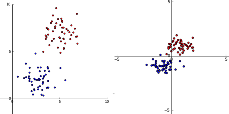
InThe $x$, each value is- and $1$ greater than the previous value, except$y$-values for each point have changed, but they are still all in the last one which issame place $2$ greaterrelative to each other. In $x_{\text{scaled}}$, aside from rounding issuesIf you look closely, each value is $0.58$ greater thanyou can see that the previous value, except forstructure of the last one whichdata is $0.58 \times 2 = 1.16$ greater. Evenidentical, even though the actual numbers have changedit has been scaled a bit, and you could go back to something that looks more like the relationship between each pairoriginal by simply 'zooming in' on the data. Because the structure of examplesthe data is the same, we say no information was lost.

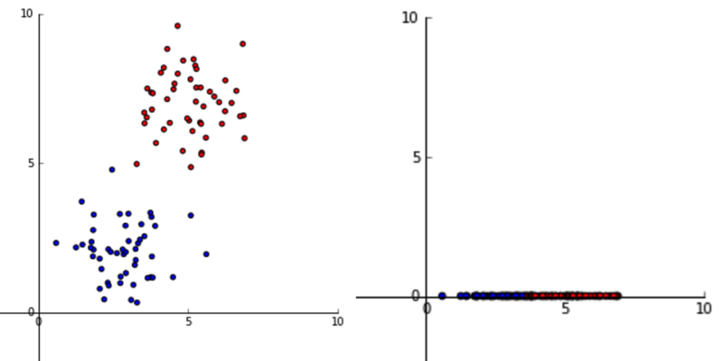
This means fromNow consider a discrimination point of viewtransformation where we only take the $x$-value, it's always just as easy for a modeland set all $y$-values to split$0$:

Original data and transformed by only keeping x-coordinate

The structure of the examples by this feature at some point usingdata has changed, and there is no way to return to the original features,data by scaling or the scaled featuresstretching space uniformly, so we say information was lost here. ForThis is an extreme example, ifbut hopefully it illustrates the first three examples belongpoint.

One way to one class, and the rest belongthink about it is to another classthink if it is more or less difficult for a classifier to distinguish between the classes after the transformation. In the first case, we can splitdraw a line that perfectly separates the two clusters just as easily with the original inputdata or the normalised data, but in the second case, there is no such line that separates the transformed data.

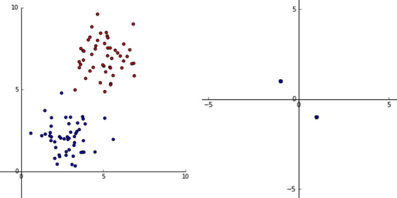
By the way, if you normalise each example rather than each feature $x$ at(as asked in your comment), for this data, you end up with something that looks like this:

Data normalised by example rather than feature

where all points land on either $3.5$$(-1,1)$ or $(1,-1)$. This makes sense, andbecause normalisation makes the range of the values span from $x_\text{scaled}$ at$-1$ to $0.17$$1$. When there are only two dimensions, one of them has to perfectly splitbecome $-1$ and the data. In other words, nohas to become $1$. Hopefully it's fairly obvious that information wasis lost in the scaling processhere, and it's generally not a good idea to do this.

This is quite a hand-wavy explanation and doesn't really cover any actual information theory concepts, but hopefully it gives you some intuition for this. If you want to dive deeper into the mathematical side of things, have a look at the Wikipedia article for information theory.

I assume by mean normalization, you mean scaling each feature by subtracting the mean and dividing by standard deviation:

$$ x_{\text{scaled}} = \frac{x - \bar{x}}{\sigma} $$

where $x$ is a feature.

Even though you are changing all of the values of $x$, they are each being scaled by the same amount - initially, a translation by a constant (subtracting the mean), and then scaling by a constant (dividing by standard deviation).

Consider some feature $x$, and its scaled version $x_\text{scaled}$:

$$ \begin{align} x &= [1,2,3,4,6] \\ x_{\text{scaled}} &= [-1.28, -0.70, -0.12, 0.46, 1.63] \end{align} $$

In $x$, each value is $1$ greater than the previous value, except for the last one which is $2$ greater. In $x_{\text{scaled}}$, aside from rounding issues, each value is $0.58$ greater than the previous value, except for the last one which is $0.58 \times 2 = 1.16$ greater. Even though the actual numbers have changed, the relationship between each pair of examples is the same.

This means from a discrimination point of view, it's always just as easy for a model to split the examples by this feature at some point using the original features, or the scaled features. For example, if the first three examples belong to one class, and the rest belong to another class, we can split the original input feature $x$ at $3.5$, and $x_\text{scaled}$ at $0.17$ to perfectly split the data. In other words, no information was lost in the scaling process.

This is quite a hand-wavy explanation and doesn't really cover any actual information theory concepts, but hopefully it gives you some intuition for this. If you want to dive deeper into the mathematical side of things, have a look at the Wikipedia article for information theory.
I assume by mean normalization, you mean scaling each feature by subtracting the mean and dividing by standard deviation:

$$ x_{\text{scaled}} = \frac{x - \bar{x}}{\sigma} $$

where $x$ is a feature.

Even though you are changing all of the values of $x$, they are each being scaled by the same amount - initially, a translation by a constant (subtracting the mean), and then scaling by a constant (dividing by standard deviation).

Here's a two-dimensional, randomly generated dataset generated with scikit-learn's make_blobs function (left) and the scaled version using the above equation for the $x$- and $y$-coordinates (right):

Original data and mean normalised data

The $x$- and $y$-values for each point have changed, but they are still all in the same place relative to each other. If you look closely, you can see that the structure of the data is identical, even though it has been scaled a bit, and you could go back to something that looks more like the original by simply 'zooming in' on the data. Because the structure of the data is the same, we say no information was lost.

Now consider a transformation where we only take the $x$-value, and set all $y$-values to $0$:

Original data and transformed by only keeping x-coordinate

The structure of the data has changed, and there is no way to return to the original data by scaling or stretching space uniformly, so we say information was lost here. This is an extreme example, but hopefully it illustrates the point.

One way to think about it is to think if it is more or less difficult for a classifier to distinguish between the classes after the transformation. In the first case, we can draw a line that perfectly separates the two clusters just as easily with the original data or the normalised data, but in the second case, there is no such line that separates the transformed data.

By the way, if you normalise each example rather than each feature (as asked in your comment), for this data, you end up with something that looks like this:

Data normalised by example rather than feature

where all points land on either $(-1,1)$ or $(1,-1)$. This makes sense, because normalisation makes the range of the values span from $-1$ to $1$. When there are only two dimensions, one of them has to become $-1$ and the other has to become $1$. Hopefully it's fairly obvious that information is lost here, and it's generally not a good idea to do this.

This is quite a hand-wavy explanation and doesn't really cover any actual information theory concepts, but hopefully it gives you some intuition for this. If you want to dive deeper into the mathematical side of things, have a look at the Wikipedia article for information theory.

Source Link
timleathart
  • 4k
  • 22
  • 35

I assume by mean normalization, you mean scaling each feature by subtracting the mean and dividing by standard deviation:

$$ x_{\text{scaled}} = \frac{x - \bar{x}}{\sigma} $$

where $x$ is a feature.

Even though you are changing all of the values of $x$, they are each being scaled by the same amount - initially, a translation by a constant (subtracting the mean), and then scaling by a constant (dividing by standard deviation).

Consider some feature $x$, and its scaled version $x_\text{scaled}$:

$$ \begin{align} x &= [1,2,3,4,6] \\ x_{\text{scaled}} &= [-1.28, -0.70, -0.12, 0.46, 1.63] \end{align} $$

In $x$, each value is $1$ greater than the previous value, except for the last one which is $2$ greater. In $x_{\text{scaled}}$, aside from rounding issues, each value is $0.58$ greater than the previous value, except for the last one which is $0.58 \times 2 = 1.16$ greater. Even though the actual numbers have changed, the relationship between each pair of examples is the same.

This means from a discrimination point of view, it's always just as easy for a model to split the examples by this feature at some point using the original features, or the scaled features. For example, if the first three examples belong to one class, and the rest belong to another class, we can split the original input feature $x$ at $3.5$, and $x_\text{scaled}$ at $0.17$ to perfectly split the data. In other words, no information was lost in the scaling process.

This is quite a hand-wavy explanation and doesn't really cover any actual information theory concepts, but hopefully it gives you some intuition for this. If you want to dive deeper into the mathematical side of things, have a look at the Wikipedia article for information theory.