Commonmark migration
Source Link

There are two solutions to this problem, though I'm only going explain the second one because I think is the best option.

##First option:

First option:

10 Scatterplots of speed of vehicle on the x-axis and predicted speed of vehicle on the y-axis. The only scenario I see this plot been useful is for clustering different types of vehicles with their speeds (if there actually are many vehicle models). Naturally you could also aggregate all data points in a single scatterplot and color-code the data set (ex. dataset1 = blue, dataset 2 = red, etc.)

Second option:

##Second option: CalculateCalculate the difference of vehicle speed and predicted speed for each data point and then bind all the results into a single data table so that each column contains the difference between actual speed and predicted speed for each data set. Then plot each column as a bar in a boxplot, here you will be able to describe all differences including signs for outliers and mean. As you might already know boxes represent standard deviation (variance) and the central line represents the mean. You can find more information about boxplots here: Wikipedia

###Sample code in R and ggplot2

Sample code in R and ggplot2

dt1 <- data.frame(data = c(runif(20, min = -1, max = 1),
                       runif(20, min = -1, max = 1), 
                       runif(20, min = -2, max = 1)), 
              datasetName = c(rep("dataset1", 20),
                              rep("dataset2", 20), 
                              rep("dataset3", 20)))


ggplot(dt1, aes(x = datasetName, y = data)) +
geom_boxplot(fill = "white", colour = "#3366FF") +
labs(x = "Dataset Name", y = "Difference Between Speed and Predicted Speed",  title = "Datasets distribution")

The resulting image should look something like this: Sample Image

There are two solutions to this problem, though I'm only going explain the second one because I think is the best option.

##First option:

10 Scatterplots of speed of vehicle on the x-axis and predicted speed of vehicle on the y-axis. The only scenario I see this plot been useful is for clustering different types of vehicles with their speeds (if there actually are many vehicle models). Naturally you could also aggregate all data points in a single scatterplot and color-code the data set (ex. dataset1 = blue, dataset 2 = red, etc.)

##Second option: Calculate the difference of vehicle speed and predicted speed for each data point and then bind all the results into a single data table so that each column contains the difference between actual speed and predicted speed for each data set. Then plot each column as a bar in a boxplot, here you will be able to describe all differences including signs for outliers and mean. As you might already know boxes represent standard deviation (variance) and the central line represents the mean. You can find more information about boxplots here: Wikipedia

###Sample code in R and ggplot2

dt1 <- data.frame(data = c(runif(20, min = -1, max = 1),
                       runif(20, min = -1, max = 1), 
                       runif(20, min = -2, max = 1)), 
              datasetName = c(rep("dataset1", 20),
                              rep("dataset2", 20), 
                              rep("dataset3", 20)))


ggplot(dt1, aes(x = datasetName, y = data)) +
geom_boxplot(fill = "white", colour = "#3366FF") +
labs(x = "Dataset Name", y = "Difference Between Speed and Predicted Speed",  title = "Datasets distribution")
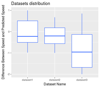
The resulting image should look something like this: Sample Image

There are two solutions to this problem, though I'm only going explain the second one because I think is the best option.

First option:

10 Scatterplots of speed of vehicle on the x-axis and predicted speed of vehicle on the y-axis. The only scenario I see this plot been useful is for clustering different types of vehicles with their speeds (if there actually are many vehicle models). Naturally you could also aggregate all data points in a single scatterplot and color-code the data set (ex. dataset1 = blue, dataset 2 = red, etc.)

Second option:

Calculate the difference of vehicle speed and predicted speed for each data point and then bind all the results into a single data table so that each column contains the difference between actual speed and predicted speed for each data set. Then plot each column as a bar in a boxplot, here you will be able to describe all differences including signs for outliers and mean. As you might already know boxes represent standard deviation (variance) and the central line represents the mean. You can find more information about boxplots here: Wikipedia

Sample code in R and ggplot2

dt1 <- data.frame(data = c(runif(20, min = -1, max = 1),
                       runif(20, min = -1, max = 1), 
                       runif(20, min = -2, max = 1)), 
              datasetName = c(rep("dataset1", 20),
                              rep("dataset2", 20), 
                              rep("dataset3", 20)))


ggplot(dt1, aes(x = datasetName, y = data)) +
geom_boxplot(fill = "white", colour = "#3366FF") +
labs(x = "Dataset Name", y = "Difference Between Speed and Predicted Speed",  title = "Datasets distribution")

The resulting image should look something like this: Sample Image

Source Link
wacax
  • 3.5k
  • 4
  • 26
  • 48

There are two solutions to this problem, though I'm only going explain the second one because I think is the best option.

##First option:

10 Scatterplots of speed of vehicle on the x-axis and predicted speed of vehicle on the y-axis. The only scenario I see this plot been useful is for clustering different types of vehicles with their speeds (if there actually are many vehicle models). Naturally you could also aggregate all data points in a single scatterplot and color-code the data set (ex. dataset1 = blue, dataset 2 = red, etc.)

##Second option: Calculate the difference of vehicle speed and predicted speed for each data point and then bind all the results into a single data table so that each column contains the difference between actual speed and predicted speed for each data set. Then plot each column as a bar in a boxplot, here you will be able to describe all differences including signs for outliers and mean. As you might already know boxes represent standard deviation (variance) and the central line represents the mean. You can find more information about boxplots here: Wikipedia

###Sample code in R and ggplot2

dt1 <- data.frame(data = c(runif(20, min = -1, max = 1),
                       runif(20, min = -1, max = 1), 
                       runif(20, min = -2, max = 1)), 
              datasetName = c(rep("dataset1", 20),
                              rep("dataset2", 20), 
                              rep("dataset3", 20)))


ggplot(dt1, aes(x = datasetName, y = data)) +
geom_boxplot(fill = "white", colour = "#3366FF") +
labs(x = "Dataset Name", y = "Difference Between Speed and Predicted Speed",  title = "Datasets distribution")

The resulting image should look something like this: Sample Image