Calculation of PCA

Question

Consider the following data set:

Now, we need to calculate the principal component analysis for this data. Here are the eigenvalues and eigenvectors calculated for the covariance matrix of this data:

So the principal component is:

Now, when I have tried to do so by hand, I have found that the eigenvalues are 1.28 and 0.0492 (which are identical to the above solution). Surely, the principal component corresponds to the eigenvalue = 1.28. However, when I tried to solve for the eigenvector, the solution was [[0] [0]] as the augmented matrix of BX=0 Was [[1 0 0] [0 1 0]]. So where is the problem here? And also how can I find the transformed data after I calculate the principle component?

Edit: the covariance matrix is

Answer 1

Before you start anything, it can be helpful to conduct some exploratory data analysis (EDA) so that you can get a general sense of the data you are working with and what you are going to be doing.

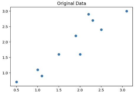
Here is a plot of the data:

It looks like there is a strong linear relationship in this dataset, so this is a strong candidate for where using PCA will likely be able to capture a large portion of the variance using only a single feature.

Method 1: By hand (sort of)

Step 1

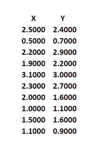
Start by converting your dataset into a matrix.

$$ \begin{array}{c|lcr} & \text{X} & \text{Y} \\ \hline 1 & 2.5 & 2.4\\ 2 & .5 & .7\\ 3 & 2.2 & 2.9\\ 4 & 1.9 & 2.2\\ 5 & 3.1 & 3.0\\ 6 & 2.3 & 2.7\\ 7 & 2.0 & 1.6\\ 8 & 1.0 & 1.1\\ 9 & 1.5 & 1.6\\ 10 & 1.1 & .9\\ \end{array} \ \ \ \ \ \ \ \ \ \ \ \ \ \ \ \ \ \ \textbf{A} = \begin{bmatrix} 2.5 & 2.4 \\ .5 & .7\\ 2.2 & 2.9\\ 1.9 & 2.2\\ 3.1 & 3.0\\ 2.3 & 2.7\\ 2.0 & 1.6\\ 1.0 & 1.1\\ 1.5 & 1.6\\ 1.1 & .9\\ \end{bmatrix} $$

Step 2

Calculate the Covariance matrix.

Recall, that this is specified by:

$$ \begin{bmatrix} Var(x) & Con(x,y) \\ Cov(x,y) & Var(y)\\ \end{bmatrix} $$

In order to calculate these values, we need to get the means $\bar{\text{X}}$ and $\bar{\text{Y}}$

$\bar{\text{X}} = { {2.5 \ + \ .5 \ + \ 2.2 \ + \ 1.9 \ + \ 3.1 \ + \ 2.3 \ + \ 2.0 \ + \ 1.0 \ + \ 1.5 \ + \ 1.1} \over {10} } = \fbox{1.81}$

$\bar{\text{Y}} = { {2.4 \ + \ .7 \ + \ 2.9 \ + \ 2.2 \ + \ 3.0 \ + \ 2.7 \ + \ 1.6 \ + \ 1.1 \ + \ 1.6 \ + \ .9} \over {10} } = \fbox{1.91}$

We calculate the values for $Var(X)$, $Var(Y)$, and $Cov(X,Y)$ below by plugging in the values to the formulas:

$Var(X) = { {\sum_{i=1}^n({x_i} - \bar{x})^2} \over {n-1} } = { {5.549} \over {9} } = \fbox{0.616555555556} $

$Var(Y) = { {\sum_{i=1}^n({y_i} - \bar{y})^2} \over {n-1} } = { {6.449} \over {9} } = \fbox{0.716555555556} $

$Cov(X,Y) = { {\sum_{i=1}^n({x_i} - \bar{x})({y_i} - \bar{y})} \over {n-1} } = { {5.539} \over {9} } = \fbox{.61544444444}$

Putting these results into the matrix, we get the Covariance matrix:

$$ \begin{bmatrix} 0.61655556 & 0.61544444 \\ 0.61544444 & 0.71655556\\ \end{bmatrix} $$

Step 3

Find the Eigen Values by taking the Eigen decomposition of the Covariance matrix.

Using the formula $A v = \lambda v$, we can rewrite it as $(A-\lambda I)v=0$ and note that this equation will have a solution at $det(A-\lambda I)=0$

$$ det = \Bigg| \begin{bmatrix} 0.61655556 & 0.61544444 \\ 0.61544444 & 0.71655556\\ \end{bmatrix} - \lambda \begin{bmatrix} 1 & 0 \\ 0 & 1 \\ \end{bmatrix} \Bigg| = 0 $$

$$ det = \Bigg| \begin{bmatrix} 0.61655556 & 0.61544444 \\ 0.61544444 & 0.71655556\\ \end{bmatrix} - \begin{bmatrix} \lambda & 0 \\ 0 & \lambda \\ \end{bmatrix} \Bigg| = 0 $$

$$ det = \Bigg| \begin{bmatrix} 0.61655556 - \lambda & 0.61544444 \\ 0.61544444 & 0.71655556 - \lambda \\ \end{bmatrix} \Bigg| = 0 $$

$$ (0.61655556 - \lambda)(0.71655556 - \lambda) \ - \ (0.61544444)(0.61544444) = $$

$$ (\lambda^2 - 1.33311112 \lambda + .441796314567 - .378771858727) = $$

$$ (\lambda^2 - 1.33311112 \lambda + .06302445584) = $$

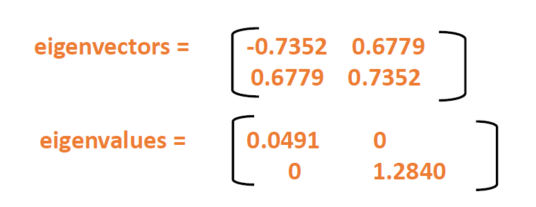
$$ \textbf{Eigen Values:} \ \lambda = \fbox{.0490834} \ \text{or} \ \lambda = \fbox{1.2840277} $$

Step 4 (Here is where we cannot really proceed solely by hand)

Find the Eigen Vectors.

For the first Eigen Vector $v_1$ for $\lambda = .0490834$

Using the formula $A v_1 = \lambda_1 v_1$

$$ \begin{bmatrix} 0.61655556 - \lambda & 0.61544444 \\ 0.61544444 & 0.71655556 - \lambda \\ \end{bmatrix} \begin{bmatrix} v_{1,1} \\ v_{1,2} \\ \end{bmatrix} = 0 $$

$$ \begin{bmatrix} 0.61655556 - .0490834 & 0.61544444 \\ 0.61544444 & 0.71655556 - .0490834 \\ \end{bmatrix} \begin{bmatrix} v_{1,1} \\ v_{1,2} \\ \end{bmatrix} = 0 $$

$$ \begin{bmatrix} .56747216 & 0.61544444 \\ 0.61544444 & .66747216 \\ \end{bmatrix} \begin{bmatrix} v_{1,1} \\ v_{1,2} \\ \end{bmatrix} = 0 $$

Note: This is not an easy equation to solve by hand! I would recommend using MATLAB here.

For the second Eigen Vector $v_2$ for $\lambda = 1.2840277$

Using the formula $A v_2 = \lambda_1 v_2$

$$ \begin{bmatrix} 0.61655556 - \lambda & 0.61544444 \\ 0.61544444 & 0.71655556 - \lambda \\ \end{bmatrix} \begin{bmatrix} v_{2,1} \\ v_{2,2} \\ \end{bmatrix} = 0 $$

$$ \begin{bmatrix} 0.61655556 - 1.2840277 & 0.61544444 \\ 0.61544444 & 0.71655556 - 1.2840277 \\ \end{bmatrix} \begin{bmatrix} v_{2,1} \\ v_{2,2} \\ \end{bmatrix} = 0 $$

$$ \begin{bmatrix} -.667477214 & 0.61544444 \\ 0.61544444 & -.61655554 \\ \end{bmatrix} \begin{bmatrix} v_{2,1} \\ v_{2,2} \\ \end{bmatrix} = 0 $$

Note: This is not an easy equation to solve by hand! I would recommend using MATLAB here.

Since it is not an easy way to solve for either of these Eigen vectors by hand, I recommend using MATLAB.

MATLAB code:

A = [0.61655556 0.61544444; 0.61544444 0.71655556]
A

[v,d]=eig(A)

v

Output:

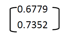
-0.735178655741955  0.677873398313764
0.677873398313764   0.735178655741955

Method 2 (using NumPy)

We can verify the results that we get above by using NumPy.

import numpy as np

# create a numpy array that stores the data matrix
matrix = np.array([[2.5, 2.4], [.5, .7], [2.2, 2.9], [1.9, 2.2], [3.1, 3.0],
                  [2.3, 2.7],[2.0, 1.6],[1.0, 1.1],[1.5, 1.6], [1.1, .9]])

# calculate the covariance matrix
covariance_matrix = np.cov(matrix[:,0], matrix[:,1])

# create variables to store the Eigen values and Eigen vectors 
eigen_values, eigen_vectors = np.linalg.eig(covariance_matrix)

Output:

Eigen Values:

array([0.0490834 , 1.28402771])

Eigen Vectors:

array([[-0.73517866, -0.6778734 ],
       [ 0.6778734 , -0.73517866]])

Method 3 (using scikit-learn)

Using the same matrix variable defined above in the NumPy example:

from sklearn.decomposition import PCA
import pandas as pd

# create and fit a PCA model
pca = PCA(n_components=2)
pca.fit(matrix)

# show the Eigen vector
pca.components_

# show the Eigen values
pca.explained_variance_

Output:

Eigen Vectors:

[[-0.6778734  -0.73517866]
 [-0.73517866  0.6778734 ]]

Eigen Values:

[1.28402771 0.0490834 ]

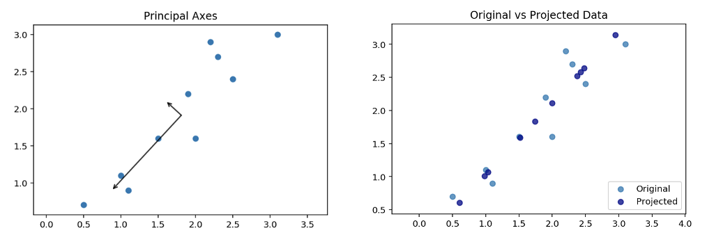
Finally, we can show plot vectors that show the direction and magnitudes of the principal axes. As you can see, the first component is longer because it explains more of the variance. We can also project the data onto the first principal component using only one feature.

Conclusion: In short, while you can calculate a good portion of this problem by hand, once you get to the part about calculating Eigen Vectors, this becomes fairly difficult. At this point, I would recommend using a computational method, such as using MATLAB, NumPy, or scikit-learn.