Great question!
tl;dr: The cell state and the hidden state are two different things, but the hidden state is dependent on the cell state and they do indeed have the same size.
Longer explanation
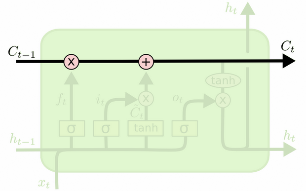
The difference between the two can be seen from the diagram below (part of the same blog):

The cell state is the bold line travelling west to east across the top. The entire green block is called the 'cell'.
The hidden state from the previous time step is treated as part of the input at the current time step.
However, it's a little harder to see the dependence between the two without doing a full walkthrough. I'll do that here, to provide another perspective, but heavily influenced by the blog. My notation will be the same, and I'll use images from the blog in my explanation.
I like to think of the order of operations a little differently from the way they were presented in the blog. Personally, like starting from the input gate. I'll present that point of view below, but please keep in mind that the blog may very well be the best way to set up an LSTM computationally and this explanation is purely conceptual.
Here's what's happening:
The input gate

The input at time $t$ is $x_t$ and $h_{t-1}$. These get concatenated and fed into a nonlinear function (in this case a sigmoid). This sigmoid function is called the 'input gate', because it acts as a stopgap for the input. It decides stochastically which values we're going to update at this timestep, based on the current input.
That is, (following your example), if we have an input vector $x_t = [1, 2, 3]$ and a previous hidden state $h_t = [4, 5, 6]$, then the input gate does the following:
a) Concatenate $x_t$ and $h_{t-1}$ to give us $[1, 2, 3, 4, 5, 6]$
b) Compute $W_i$ times the concatenated vector and add the bias (in math: $W_i \cdot [x_t, h_{t-1}] + b_i$, where $W_i$ is the weight matrix from the input vector to the nonlinearity; $b_i$ is the input bias).
Let's assume we're going from a six-dimensional input (the length of the concatenated input vector) to a three-dimensional decision on what states to update. That means we need a 3x6 weight matrix and a 3x1 bias vector. Let's give those some values:
$W_i = \begin{bmatrix} 1 & 1 & 1 & 1 & 1 & 1 \\ 2 & 2 & 2 & 2 & 2 & 2 \\ 3 & 3 & 3 & 3 & 3 & 3\end{bmatrix}$
$b_i = \begin{bmatrix} 1 \\ 1 \\ 1 \end{bmatrix}$
The computation would be:
$\begin{bmatrix} 1 & 1 & 1 & 1 & 1 & 1 \\ 2 & 2 & 2 & 2 & 2 & 2 \\ 3 & 3 & 3 & 3 & 3 & 3\end{bmatrix} \cdot \begin{bmatrix} 1 \\ 2 \\ 3 \\ 4 \\5 \\6 \end{bmatrix} + \begin{bmatrix} 1 \\ 1 \\ 1 \end{bmatrix} = \begin{bmatrix} 22 \\ 42 \\ 62 \end{bmatrix}$
c) Feed that previous computation into a nonlinearity: $i_t = \sigma (W_i \cdot [x_t, h_{t-1}] + b_i)$
$\sigma(x) = \frac{1}{1 + exp(-x)}$ (we apply this elementwise to the values in the vector $x$)
$\sigma(\begin{bmatrix} 22 \\ 42 \\ 62 \end{bmatrix}) = [\frac{1}{1 + exp(-22)}, \frac{1}{1 + exp(-42)}, \frac{1}{1 + exp(-62)}] = [1, 1, 1]$
In English, that means we're going to update all of our states.
The input gate has a second part:
d) $\tilde{C_t} = tanh(W_C[x_t, h_{t-1}] + b_C)$
The point of this part is to compute how we would update the state, if we were to do so. It's the contribution from the new input at this time step to the cell state. The computation follows the same procedure illustrated above, but with a tanh unit instead of a sigmoid unit.
The output $\tilde{C_t}$ is multiplied by that binary vector $i_t$, but we'll cover that when we get to the cell update.
Together, $i_t$ tells us which states we want to update, and $\tilde{C_t}$ tells us how we want to update them. It tells us what new information we want to add to our representation so far.
Then comes the forget gate, which was the crux of your question.
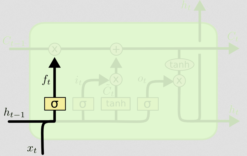
The forget gate

The purpose of the forget gate is to remove previously-learned information that is no longer relevant. The example given in the blog is language-based, but we can also think of a sliding window. If you're modelling a time series that is naturally represented by integers, like counts of infectious individuals in an area during a disease outbreak, then perhaps once the disease has died out in an area, you no longer want to bother considering that area when thinking about how the disease will travel next.
Just like the input layer, the forget layer takes the hidden state from the previous time step and the new input from the current time step and concatenates them. The point is to decide stochastically what to forget and what to remember. In the previous computation, I showed a sigmoid layer output of all 1's, but in reality it was closer to 0.999 and I rounded up.
The computation looks a lot like what we did in the input layer:
$f_t = \sigma(W_f [x_t, h_{t-1}] + b_f)$
This will give us a vector of size 3 with values between 0 and 1. Let's pretend it gave us:
$[0.5, 0.8, 0.9]$
Then we decide stochastically based on these values which of those three parts of information to forget. One way of doing this is to generate a number from a uniform(0, 1) distribution and if that number is less than the probability of the unit 'turning on' (0.5, 0.8, and 0.9 for units 1, 2, and 3 respectively), then we turn that unit on. In this case, that would mean we forget that information.
Quick note: the input layer and the forget layer are independent. If I were a betting person, I'd bet that's a good place for parallelization.
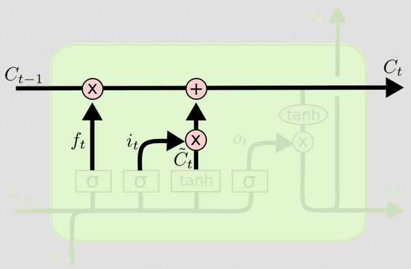
Updating the cell state

Now we have all we need to update the cell state. We take a combination of the information from the input and the forget gates:
$C_t = f_t \circ C_{t-1} + i_t \circ \tilde{C_t}$
Now, this is going to be a little odd. Instead of multiplying like we've done before, here $\circ$ indicates the Hadamard product, which is an entry-wise product.
Aside: Hadamard product
For example, if we had two vectors $x_1 = [1, 2, 3]$ and $x_2 = [3, 2, 1]$ and we wanted to take the Hadamard product, we'd do this:
$x_1 \circ x_2 = [(1 \cdot 3), (2 \cdot 2), (3 \cdot 1)] = [3, 4, 3]$
End Aside.
In this way, we combine what we want to add to the cell state (input) with what we want to take away from the cell state (forget). The result is the new cell state.
The output gate

This will give us the new hidden state. Essentially the point of the output gate is to decide what information we want the next part of the model to take into account when updating the subsequent cell state. The example in the blog is again, language: if the noun is plural, the verb conjugation in the next step will change. In a disease model, if the susceptibility of individuals in a particular area is different than in another area, then the probability of acquiring an infection may change.
The output layer takes the same input again, but then considers the updated cell state:
$o_t = \sigma(W_o [x_t, h_{t-1}] + b_o)$
Again, this gives us a vector of probabilities. Then we compute:
$h_t = o_t \circ tanh(C_t)$
So the current cell state and the output gate must agree on what to output.
That is, if the result of $tanh(C_t)$ is $[0, 1, 1]$ after the stochastic decision has been made as to whether each unit is on or off, and the result of $o_t$ is $[0, 0, 1]$, then when we take the Hadamard product, we're going to get $[0, 0, 1]$, and only the units that were turned on by both the output gate and in the cell state will be part of the final output.
[EDIT: There's a comment on the blog that says the $h_t$ is transformed again to an actual output by $y_t = \sigma(W \cdot h_t)$, meaning that the actual output to the screen (assuming you have some) is the result of another nonlinear transformation.]
The diagram shows that $h_t$ goes to two places: the next cell, and to the 'output' - to the screen. I think that second part is optional.
There are a lot of variants on LSTMs, but that covers the essentials!

