How to interpert ResNet50 Layer Types

Question

I am trying to recreate the ResNet50 from scratch, but I don't quite understand how to interpret the matrices for the layers.

For instance: [[1x1,64] [3x3, 64] [1x1, 4]] x 3

I know it's supposed to be a convolution layer but what do each of the numbers represent?

Answer 1

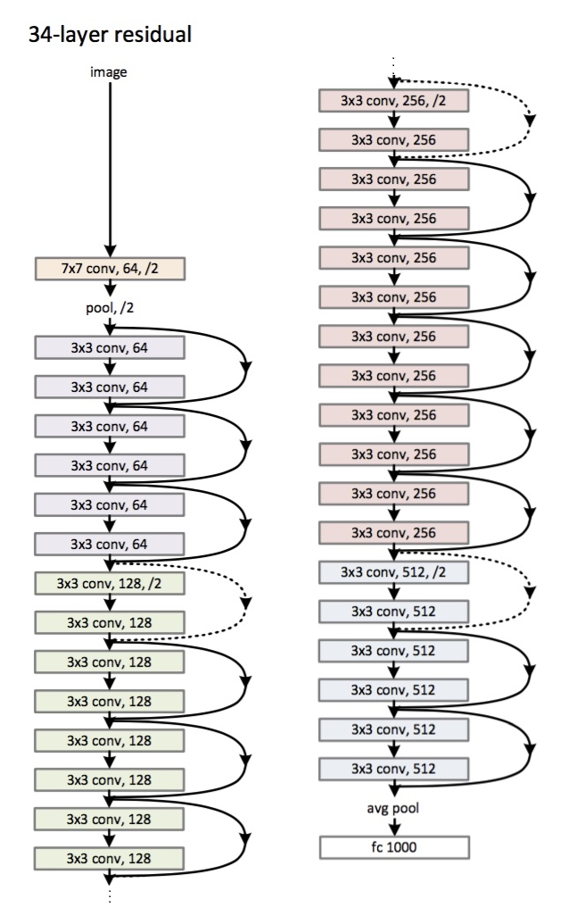
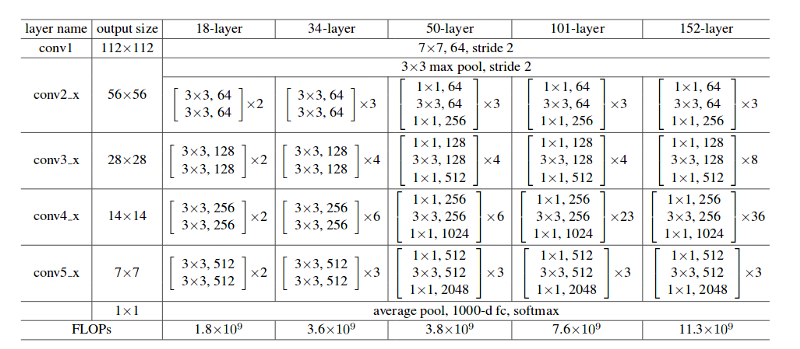
In order to make the explanation clear I will use the example of 34-layers:

• First you have a convolutional layer with 64 filters and kernel size of 7x7 (conv1 in your table) followed by a max pooling layer. Note that the stride is specified to be stride = 2 in both cases.

• Next, in conv2_x you have the mentioned pooling layer and the following convolution layers. Here the layers are normally grouped in pairs (trios in bigger architectures) because is how the residuals are connected (the arrows jumping each two layers). The first matrix:

  \begin{equation}\begin{bmatrix} 3x3, & 64 \\ 3x3, & 64 \end{bmatrix}*3\end{equation}

means that you have 2 layers of kernel_size = 3x3, num_filters = 64 and these are repeated x3. These correspond to the layers between pool,/2 and the filter 128 ones, 6 layers in total (one pair times 3).

• Following, we have conv3_x:

  \begin{equation}\begin{bmatrix} 3x3, & 128 \\ 3x3, & 128 \end{bmatrix}*4\end{equation}

2 layers of kernel_size = 3x3, num_filters = 128 and these are also repeated but on this occasion times 4. These are the following 8 green layers in the figure.

This continues until the avg_pooling and the softmax.

Be aware that the stride is always 1 except when the filter size increases. This is discusssed in the paper:

Plain Network: Our plain baselines are mainly inspired by the philosophy of VGG nets. The convolutional layers mostly have 3×3 filters and follow two simple design rules: (i) for the same output feature map size, the layers have the same number of filters; and (ii) if the feature map size is halved, the number of filters is doubled so as to preserve the time complexity per layer. We perform downsampling directly by convolutional layers that have a stride of 2.

Residual Networks: The baseline architectures are the same as the above plain nets, expect that a shortcut connection is added to each pair of 3×3 filters.

That is why, each time the number of filters is doubled you will see that the first layer of a different colour specifies num_filters/2.

Answer 2

Your example doesn't refer to a convolutional layer, but a stack of convolutional layers that create a residual block.

Per Table 1 in the original paper, here is an example residual block with some notation:

$[{\text{N x N, C}_1\atop\text{M x M, C}_2}] \text{ x L} $

• $\text{N x N}$ and $\text{M x M}$ specify the size of the kernel used in that layer. In the paper the authors call them filters.
• $\text{C}_1$ and $\text{C}_2$ refer to the number of channels in that convolutional layer.
• $\text{L}$ is the number of times this block is repeated for that residual layer.

Good luck, hope this helps!

Answer 3

I hope this notebook will help you to understand better. The implementation is in Keras so it's quick grasp!