4
$\begingroup$

I'm reading the book Introduction to Data Mining by Tan, Steinbeck, and Kumar. In the chapter on Decision Trees, when talking about the "Methods for Expressing Attribute Test Conditions" the book says :

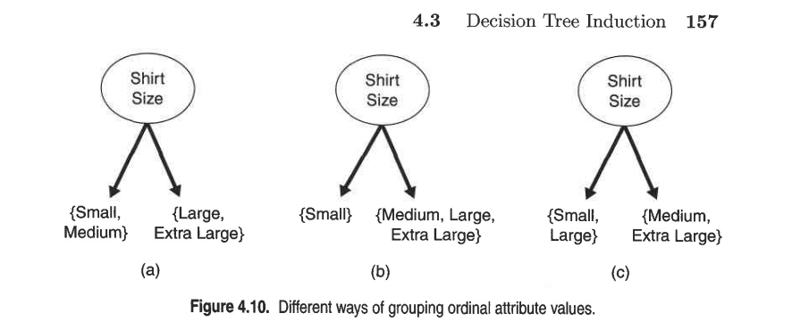
"Ordinal attributes can also produce binary or multiway splits. Ordinal attribute values can be grouped as long as the grouping does not violate the order property of the attribute values. Figure 4.10 illustrates various ways of splitting training records based on the Shirt Size attribute. The groupings shown in Figures 4.10(a) and (b) preserve the order among the attribute values, whereas the grouping shown in Figure a.10(c) violates this property because it combines the attribute values Small and Large into the same partition while Medium and Extra Large are combined into another partition."

enter image description here

Why ordinal attribute values can be grouped as long as the grouping does not violate the order property of the attribute values?

$\endgroup$

2 Answers 2

3
$\begingroup$

I'd say the distinct handling of the ordered and unordered factor in decision trees is more convention and implementation detail than a necessity.

But it is also an important optimization feature. See the documentation of the rpart here

We have said that for a categorical predictor with $m$ levels, all $2^{(m-1)}$ different possible splits are tested..

and

Luckily, for any ordered outcome there is a computational shortcut that allows the program to find the best split using only $m-1$ comparisons.

As you see, the ordered factor may be processed much effectively.

My advice therefore - as a part of the feature ingeneering decide whether to use a factor ordered or unordered:

Use ordered factor only if it is highly correlated with the output variable, otherwise fall back to an unordered factor

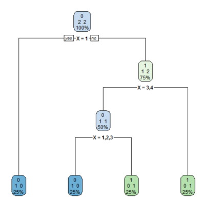
Bellow is a simple example, how can a scattered output variable with an ordered factor as a feature fool the decision treee to be very deep and ineffective.

> df
  X Y
1 1 0
2 2 1
3 3 0
4 4 1
> str(df)
'data.frame':   4 obs. of  2 variables:
 $ X: Ord.factor w/ 4 levels "1"<"2"<"3"<"4": 1 2 3 4
 $ Y: num  0 1 0 1

Notice that the output variable $Y$ is highly uncorrelated with the ordered factor.

> fit <- rpart(Y ~ X, method="class", data = df, control=rpart.control(minsplit = 1))  
> print(fit)
n= 4 

node), split, n, loss, yval, (yprob)
      * denotes terminal node

 1) root 4 2 0 (0.50000000 0.50000000)  
   2) X=1 1 0 0 (1.00000000 0.00000000) *
   3) X=2,3,4 3 1 1 (0.33333333 0.66666667)  
     6) X=3,4 2 1 0 (0.50000000 0.50000000)  
      12) X=1,2,3 1 0 0 (1.00000000 0.00000000) *
      13) X=4 1 0 1 (0.00000000 1.00000000) *
     7) X=1,2 1 0 1 (0.00000000 1.00000000) *

Which leads to a deep (and unscalable) decision tree.
enter image description here

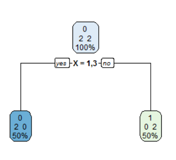
Making the factor unordered results in the optimal decision tree.

> df
  X Y
1 1 0
2 2 1
3 3 0
4 4 1
> str(df)
'data.frame':   4 obs. of  2 variables:
 $ X: Factor w/ 4 levels "1","2","3","4": 1 2 3 4
 $ Y: num  0 1 0 1
> 

> fit <- rpart(Y ~ X, method="class", data = df, control=rpart.control(minsplit = 1))  
> print(fit)
n= 4 

node), split, n, loss, yval, (yprob)
      * denotes terminal node

1) root 4 2 0 (0.50000000 0.50000000)  
  2) X=1,3 2 0 0 (1.00000000 0.00000000) *
  3) X=2,4 2 0 1 (0.00000000 1.00000000) *
enter image description here

$\endgroup$
1
$\begingroup$

I guess the reason is clear. We usually split things into specified parts which are not contradictory. A special thing can be small and medium, as one group, and large, as the other group. But it cannot be small and large at the same time. The point is that you have a sequence in your data. If there was no such thing you could have different combinations of attribute values. Suppose you have a set of attribute values for a fruit. It can be apple, pineapple and watermelon. Due to the fact that there is no ordinal, you can have all possible combination for binary splits; in the previous case, you can not because your binary split somehow violates the logical sequence.

$\endgroup$
5
  • $\begingroup$ To me is useless, since for example a T-shirt factory can decide to print red tshirts of size Small and Large and blue tshirts of sizes medium and extralarge. Since we don't know the model that generates the data how can we infer that it's "better" to preserve the order in the splits of a ordinal attribute ? $\endgroup$
    – Koinos
    Commented Aug 1, 2018 at 12:06
  • $\begingroup$ Well@Koinos, feature construction is one of the important tasks of the modeler. It is up to you to decide whether to represent a categorical veriable as ordered or unordered. $\endgroup$
    – Michael M
    Commented Aug 1, 2018 at 12:13
  • $\begingroup$ I don't grab the advantages of maintaining the order of an attribute splits... $\endgroup$
    – Koinos
    Commented Aug 1, 2018 at 12:23
  • $\begingroup$ @Koinos in the example that you have provided, actually you are not preserving the order and your ordinal attribute is actually more nominal. Since we don't know the model that generates the data how can we infer that it's "better" to preserve the order in the splits of a ordinal attribute ?. Well, this is not true entirely due to the fact that we have the data and we can have assumptions about the distribution of data. Moreover, there are approaches to findout it's better to have binary or multiway splits. $\endgroup$ Commented Aug 1, 2018 at 12:41
  • $\begingroup$ For binary, depnding on your information criterion, such as Gini, Information Gain or maybe Gain Ratio, you as the ML practitioner have to find out the best part to split. But one of the things that can get complicated is that ordinal features may be used multiple times for a path from the root to a leaf. In that way, if you don't preseverve the order, it can get so much complicated. $\endgroup$ Commented Aug 1, 2018 at 12:41

Your Answer

By clicking “Post Your Answer”, you agree to our terms of service and acknowledge you have read our privacy policy.

Not the answer you're looking for? Browse other questions tagged or ask your own question.