Convolutions from a DSP perspective
I'm a bit late to this but still would like to share my perspective and insights. My background is theoretical physics and digital signal processing. In particular I studied wavelets and convolutions are almost in my backbone ;)
The way people in the deep learning community talk about convolutions was also confusing to me. From my perspective what seems to be missing is a proper separation of concerns. I will explain the deep learning convolutions using some DSP tools.
Disclaimer
My explanations will be a bit hand-wavy and not mathematical rigorous in order to get the main points across.
Definitions
Let's define a few things first. I limit my discussion to one dimensional (the extension to more dimension is straight forward) infinite (so we don't need to mess with boundaries) sequences $x_n = \{x_n\}_{n=-\infty}^{\infty} = \{\dots, x_{-1}, x_{0}, x_{1}, \dots \}$.
A pure (discrete) convolution between two sequences $y_n$ and $x_n$ is defined as
$$ (y * x)_n = \sum_{k=-\infty}^{\infty} y_{n-k} x_k $$
If we write this in terms of matrix vector operations it looks like this (assuming a simple kernel $\mathbf{q} = (q_0,q_1,q_2)$ and vector $\mathbf{x} = (x_0, x_1, x_2, x_3)^T$):
$$ \mathbf{q} * \mathbf{x} =
\left( \begin{array}{cccc}
q_1 & q_0 & 0 & 0 \\
q_2 & q_1 & q_0 & 0 \\
0 & q_2 & q_1 & q_0 \\
0 & 0 & q_2 & q_1 \\
\end{array} \right)
\left( \begin{array}{cccc}
x_0 \\ x_1 \\ x_2 \\ x_3
\end{array} \right)
$$
Let's introduce the down- and up-sampling operators, $\downarrow$ and $\uparrow$, respectively. Downsampling by factor $k \in \mathbb{N}$ is removing all samples except every k-th one:
$$ \downarrow_k\!x_n = x_{nk} $$
And upsampling by factor $k$ is interleaving $k-1$ zeros between the samples:
$$ \uparrow_k\!x_n = \left \{ \begin{array}{ll}
x_{n/k} & n/k \in \mathbb{Z} \\
0 & \text{otherwise}
\end{array} \right.
$$
E.g. we have for $k=3$:
$$ \downarrow_3\!\{ \dots, x_0, x_1, x_2, x_3, x_4, x_5, x_6, \dots \} = \{ \dots, x_0, x_3, x_6, \dots \} $$
$$ \uparrow_3\!\{ \dots, x_0, x_1, x_2, \dots \} = \{ \dots x_0, 0, 0, x_1, 0, 0, x_2, 0, 0, \dots \} $$
or written in terms of matrix operations (here $k=2$):
$$ \downarrow_2\!x =
\left( \begin{array}{cc}
x_0 \\ x_2
\end{array} \right) =
\left( \begin{array}{cccc}
1 & 0 & 0 & 0 \\
0 & 0 & 1 & 0 \\
\end{array} \right)
\left( \begin{array}{cccc}
x_0 \\ x_1 \\ x_2 \\ x_3
\end{array} \right)
$$
and
$$ \uparrow_2\!x =
\left( \begin{array}{cccc}
x_0 \\ 0 \\ x_1 \\ 0
\end{array} \right) =
\left( \begin{array}{cc}
1 & 0 \\
0 & 0 \\
0 & 1 \\
0 & 0 \\
\end{array} \right)
\left( \begin{array}{cc}
x_0 \\ x_1
\end{array} \right)
$$
As one can already see, the down- and up-sample operators are mutually transposed, i.e. $\uparrow_k = \downarrow_k^T$.
Deep Learning Convolutions by Parts
Let's look at the typical convolutions used in deep learning and how we write them. Given some kernel $\mathbf{q}$ and vector $\mathbf{x}$ we have the following:
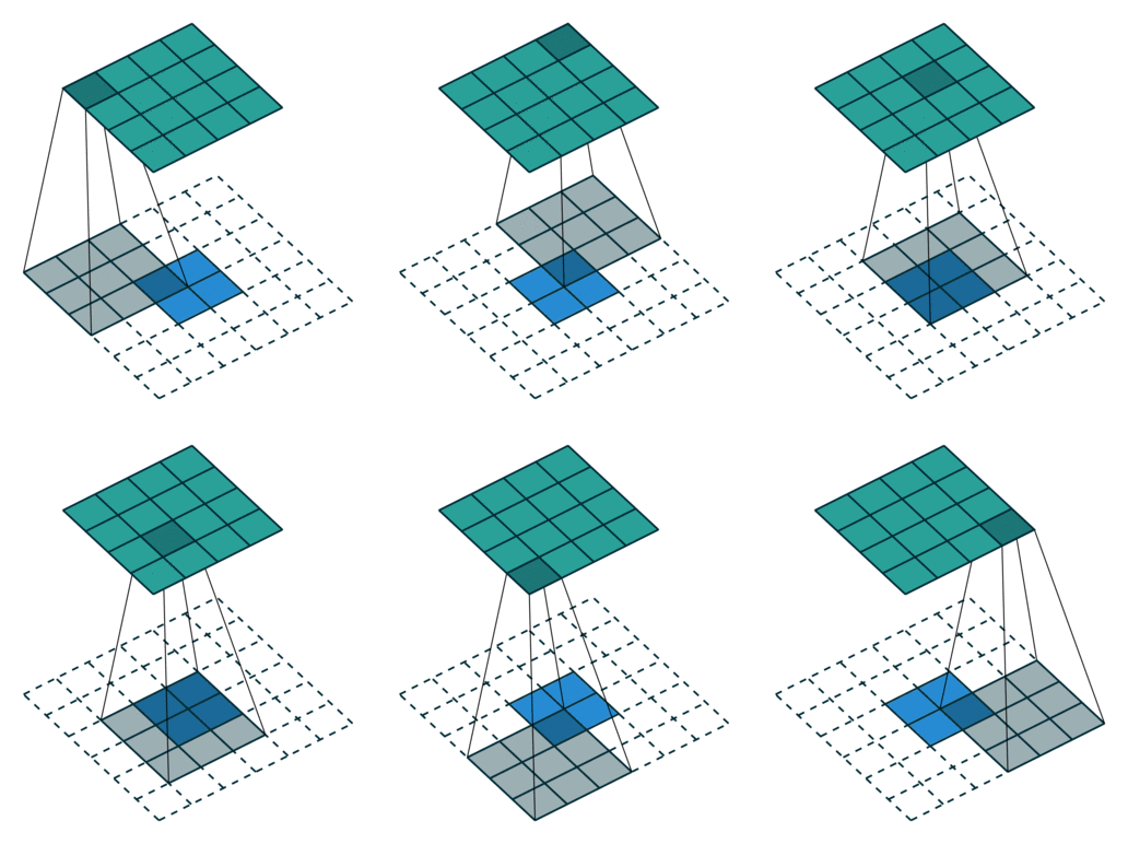
- a strided convolution with stride $k$ is $\downarrow_k\!(\mathbf{q} * \mathbf{x})$,
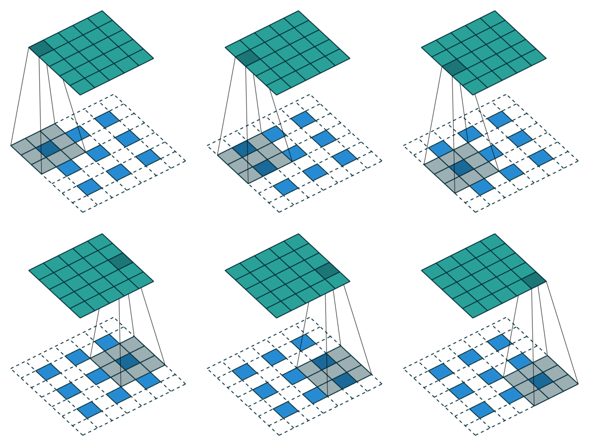
- a dilated convolution with factor $k$ is $(\uparrow_k\!\mathbf{q}) * \mathbf{x}$,
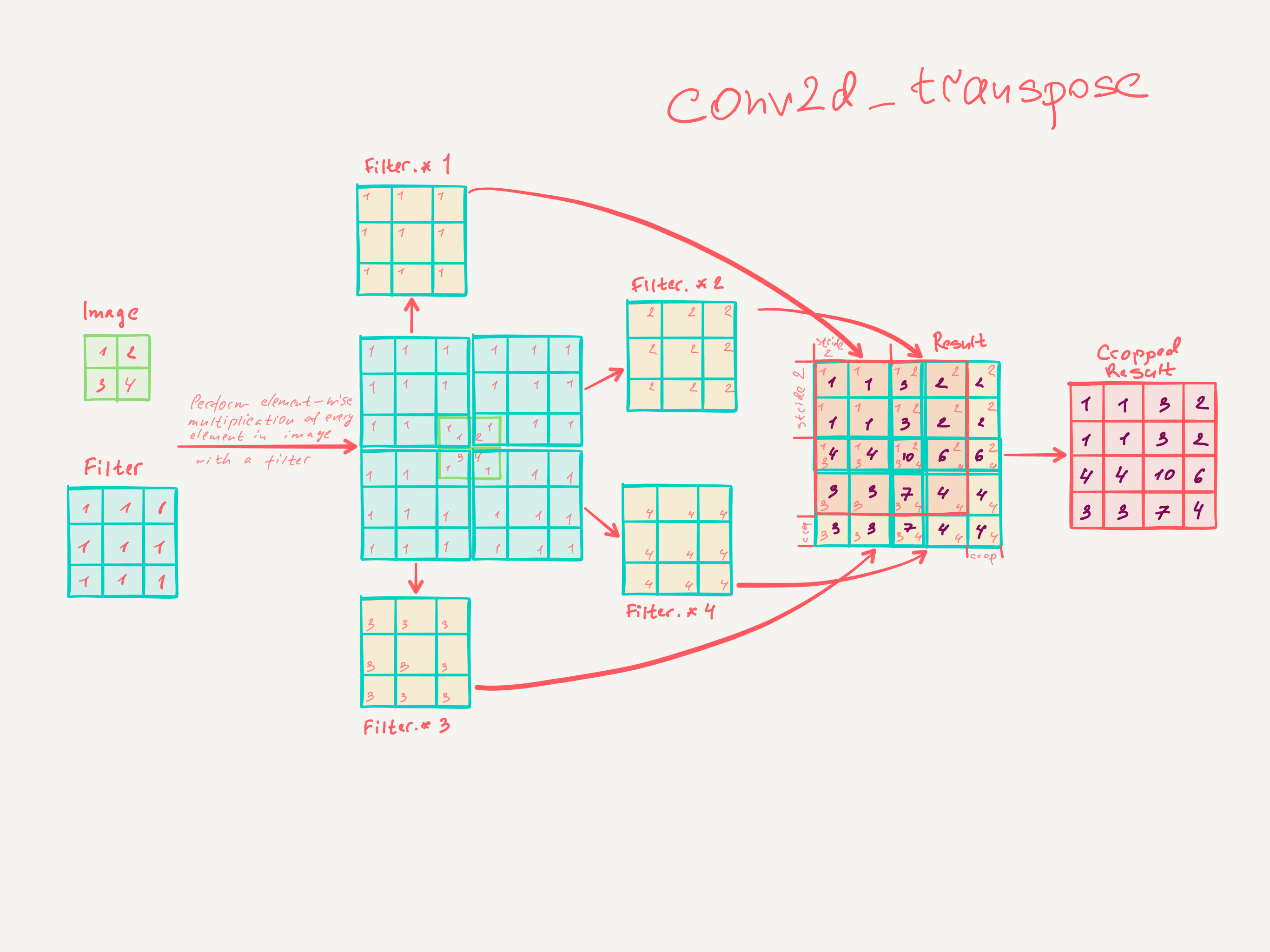
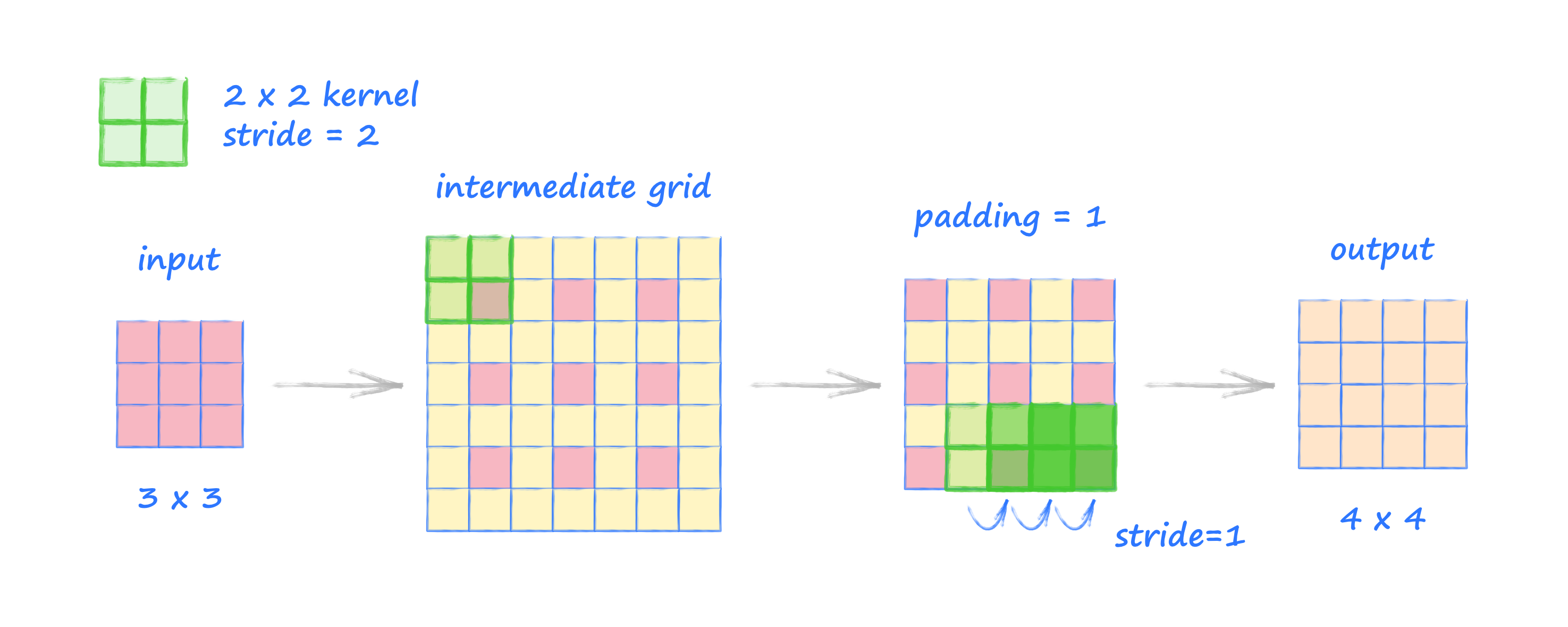
- a transposed convolution with stride $k$ is $ \mathbf{q} * (\uparrow_k\!\mathbf{x})$
Let's rearrange the transposed convolution a bit:
$$
\mathbf{q} * (\uparrow_k\!\mathbf{x}) \; = \;
\mathbf{q} * (\downarrow_k^T\!\mathbf{x}) \; = \;
(\uparrow_k\!(\mathbf{q}*)^T)^T\mathbf{x}
$$
In this notation $(\mathbf{q}*)$ must be read as an operator, i.e. it abstracts convolving something with kernel $\mathbf{q}$.
Or written in matrix operations (example):
$$
\begin{align}
\mathbf{q} * (\uparrow_k\!\mathbf{x}) & =
\left( \begin{array}{cccc}
q_1 & q_0 & 0 & 0 \\
q_2 & q_1 & q_0 & 0 \\
0 & q_2 & q_1 & q_0 \\
0 & 0 & q_2 & q_1 \\
\end{array} \right)
\left( \begin{array}{cc}
1 & 0 \\
0 & 0 \\
0 & 1 \\
0 & 0 \\
\end{array} \right)
\left( \begin{array}{c}
x_0\\
x_1\\
\end{array} \right)
\\ & =
\left( \begin{array}{cccc}
q_1 & q_2 & 0 & 0 \\
q_0 & q_1 & q_2 & 0 \\
0 & q_0 & q_1 & q_2 \\
0 & 0 & q_0 & q_1 \\
\end{array} \right)^T
\left( \begin{array}{cccc}
1 & 0 & 0 & 0\\
0 & 0 & 1 & 0\\
\end{array} \right)^T
\left( \begin{array}{c}
x_0\\
x_1\\
\end{array} \right)
\\ & =
\left(
\left( \begin{array}{cccc}
1 & 0 & 0 & 0\\
0 & 0 & 1 & 0\\
\end{array} \right)
\left( \begin{array}{cccc}
q_1 & q_2 & 0 & 0 \\
q_0 & q_1 & q_2 & 0 \\
0 & q_0 & q_1 & q_2 \\
0 & 0 & q_0 & q_1 \\
\end{array} \right)
\right)^T
\left( \begin{array}{c}
x_0\\
x_1\\
\end{array} \right)
\\ & = (\uparrow_k\!(\mathbf{q}*)^T)^T\mathbf{x}
\end{align}
$$
As one can see the is the transposed operation, thus, the name.
Connection to Nearest Neighbor Upsampling
Another common approach found in convolutional networks is upsampling with some built-in form of interpolation. Let's take upsampling by factor 2 with a simple repeat interpolation.
This can be written as $\uparrow_2\!(1\;1) * \mathbf{x}$. If we also add a learnable kernel $\mathbf{q}$ to this we have $\uparrow_2\!(1\;1) * \mathbf{q} * \mathbf{x}$. The convolutions can be combined, e.g. for $\mathbf{q}=(q_0\;q_1\;q_2)$, we have $$(1\;1) * \mathbf{q} = (q_0\;\;q_0\!\!+\!q_1\;\;q_1\!\!+\!q_2\;\;q_2),$$
i.e. we can replace a repeat upsampler with factor 2 and a convolution with a kernel of size 3 by a transposed convolution with kernel size 4. This transposed convolution has the same "interpolation capacity" but would be able to learn better matching interpolations.
Conclusions and Final Remarks
I hope I could clarify some common convolutions found in deep learning a bit by taking them apart in the fundamental operations.
I didn't cover pooling here. But this is just a nonlinear downsampler and can be treated within this notation as well.

