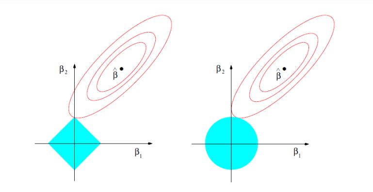
These diagrams show the "constrained" version of lasso/ridge, in which you minimize the pure loss function subject to a constraint $\|\beta\|_1\leq t$ or $\|\beta\|_2\leq t$. (Another common version adds a penalty to the loss, and these are equivalent.)
The bluish solid shapes are the set of points with $\|\beta\|\leq t$, on the left with L1 norm and on the right with L2 norm. $\hat{\beta}$ represents the unpenalized optimum value of $\beta$, and the ovals around it are the level curves of the loss function.
We know that the optimum constrained solution will occur at a point of tangency of the level curves of the loss function and the constraint boundary, specifically with the "smallest" level curve that touches the constraint region. Then the point of the picture is that, with the pointy L1 constraint, you are much more likely for that point of tangency to occur at one of the corners, which correspond to one (or more, if we try to generalize to higher dimensions) of the coordinates in $\beta$ being zero. Compare to the L2 boundary, where the tangency being exactly along one of the axes is much less likely.

