Problems to understand how to create the input data for time series forecasting with a recurrent neural network in Keras

Question

I just started to use recurrent neural networks (RNN) with Keras for time-series forecasting and I found this tutorial Forecasting with RNN. I have difficulties understanding how to build the training data both regarding the syntax and the format of the input data.

Here is the code:

import pandas as pd
import numpy as np
import tensorflow as tf

from tensorflow import keras
from matplotlib import pyplot as plt

# Read the data for the parameters from a csv file
df = pd.read_csv("C:/Users/Python/Data/tutorial_electricityPrice.csv", sep =",")

#Delete the first column as it is not used in the tutorial for forecasting
del df['datetime']


data = df.values

n_steps = 168

series_reshaped =  np.array([data[i:i + (n_steps+24)].copy() for i in range(len(data) - (n_steps+24))])


X_train = series_reshaped[:43800, :n_steps] 
X_valid = series_reshaped[43800:52560, :n_steps] 
X_test = series_reshaped[52560:, :n_steps] 
Y = np.empty((61134, n_steps, 24))  
for step_ahead in range(1, 24 + 1):     
    Y[..., step_ahead - 1] =   series_reshaped[..., step_ahead:step_ahead + n_steps, 0]
  
Y_train = Y[:43800] 
Y_valid = Y[43800:52560] 
Y_test = Y[52560:]

np.random.seed(42)
tf.random.set_seed(42)

model6 = keras.models.Sequential([
    keras.layers.SimpleRNN(20, return_sequences=True, input_shape=[None, 6]),
    keras.layers.SimpleRNN(20, return_sequences=True),
    keras.layers.TimeDistributed(keras.layers.Dense(24))
])

model6.compile(loss="mean_squared_error", optimizer="adam", metrics=['mean_absolute_percentage_error'])
history = model6.fit(X_train, Y_train, epochs=10,batch_size=64,
                    validation_data=(X_valid, Y_valid))

So in this case, 168 hours of the past are used (n_steps) to make a prediction for the next 24 hours of electricity prices. 6 features are used.

I have problems both understanding the format and the syntax for creating the input data of the RNN.

Format question

I uploaded a screenshot of the dimensions of the data-arrays from Spyder:

So basically we have the full data array 'series_reshaped' with the size (61134, 192, 6). Then we have the input data X_train with the size (43800, 168, 6). The first dimension is the timeslot, the second dimension is the past timeslots that are used for prediction and the third dimension is the 6 features for every of the 168 past timeslots. Then we have the labels Y_train with the size (43800, 168, 24). Here I do not understand why we have 168 in the second dimension. As far as I understood for each of the 168 past values * 6 features of the input data, we have 24 target values. So why is the second dimension then not 168*6 = 1008? Because we have a mapping of 1008 inputs to 24 outputs?

Syntax question

I do not really understand how these lines work in Python:

for step_ahead in range(1, 24 + 1):     
    Y[..., step_ahead - 1] =   series_reshaped[..., step_ahead:step_ahead + n_steps, 0]

• Why does this create a Y array of the dimension (61134, 168, 24) or transfer the correct data into it?
• The index step_ahead only takes values from 1 to 24 and now we assign to 24 entries of the second dimension of the array Y 168 values from the past values of the series_reshaped. So why do we only assign the values to the 24 entries of the second dimension of Y and not to the full 168 entries?
• And why are we looking into the past data of the series_reshaped array (second dimension)? For me, these lines are extremely confusing although they apparently do the right thing. Can anyone tell me a little bit more about the syntax of those lines?

Generally, I'd appreciate every comment and would be quite thankful for your help.

---

Update

Related questions: Hi all, as I still have problems with those questions I would like to ask some related questions:

1. About the creation of the input data: how can I know which structure the input data should have? And how can I then derive something like this code

for step_ahead in range(1, 24 + 1):
    Y[..., step_ahead - 1] = series_reshaped[..., step_ahead:step_ahead + n_steps, 0]

2. At the end of the training in the tutorial they use the following code for the prediction

Y_pred = model6.predict(X_test)

last_list=[]

for i in range (0, len(Y_pred)):
  last_list.append((Y_pred[i][0][23]))

So they take Y_pred[i][0][23] to construct the 1-dimensional list with the predicted values. Why do they take [0][23] and not for example [1][14]? They want to predict 24 hours in advance. Can I just always take Y_pred[i][0][23]?

3. I still do not understand one of my initial questions: Why is the labeled dataset Y for training [Batch, 168, 24] if return_sequence =true? We use the past 168 values to forecast 24 hours. We use 168*6 features for forecasting. For each element in the batch (each timeslot) we then have an output of 24 hours. So we should have the training data with dimension [Batch, 24] and not [Batch, 168, 24]. For every timeslot in the batch, we need 168 past values. How is it then possible to map 24 hours of predictions to every 168 of the past values?

Reminder: My bounty expires in three days and unfortunately I have not received another more comprehensive answer. I'd highly appreciate any new answer that might explain the input data for time series forecasting with a recurrent neural network.

Answer 1

You should look at the data with Features intact for each step.Featues can't be flattened since each point of time is defined by all the Features.
Let's see this snap,

The upper table is the data
Let's assume we want to predict 2 steps using 3 input steps.

So, one instance of our input will have 3 sequential steps having 6 Features part of each sequential steps. So, input becomes [Batch, 3, 6]. In you case [Batch, 168, 6]

Output need to have 2 sequential steps(per requirement). Since we are predicting one feature, so it will have just one feature. So, output shape [Batch, 2]. In your case [Batch, 24].
But this would have been the case when we only want the backprop after the last step i.e. return_sequences=False for the last RNN.
Since we are returning sequence every time, so output must have 24 values for each sequential step. So output becomes [Batch, 168, 24]

Features

Features don't pass sequentially, all 6 Features will pass together for each time step. Check this depiction below.
Each feature will go into each Neuron and each neuron will add a recurrent weight to each Neuron. If you check your model's parameter count for the first layer, it will be 540.
6*20(Input weights) + 20*20(Recurrent) + 20(Bias) = 540

$\hspace{5cm}$ ^{Image credit - SO Answer}

Answer 2

I'm late for this post. Let's break down the problem into manageable parts and address each question. I'll provide insights into the format, syntax, and logic of your code.

1. Format Question: Understanding Dimensions

Why is Y_train shaped (43800, 168, 24) and not (43800, 1008, 24)?

The confusion arises from a misunderstanding of how the input data (X_train) and target labels (Y_train) are structured. Here's the breakdown:

• input data X_train (43800, 168, 6):

  Each sample in the batch (43800 timeslots) consists of 168 time steps (n_steps) of historical data. For each of these time steps, 6 features (e.g., temperature, wind speed, etc.) are provided.

• target labels Y_train (43800, 168, 24):

  Here, the second dimension (168) aligns with the 168 time steps of X_train. For each of these 168 time steps, we predict 24 future values (for each time step, we aim to forecast the next 24 hours).

  The key point is that the RNN is configured to predict 24 future steps for each of the 168 input time steps. This explains why Y_train has the shape (43800, 168, 24).

If we wanted the model to predict only 24 future values for the entire 168-step input sequence (rather than for each time step within the sequence), then Y_train would have been (43800, 24).

---

2. Syntax Question: Code Analysis

for step_ahead in range(1, 24 + 1):
   Y[..., step_ahead - 1] = series_reshaped[..., step_ahead:step_ahead + n_steps, 0]

Let's break it down step-by-step:

• range(1, 24 + 1):

  • Loops from 1 to 24 (inclusive), where each value represents the future step to predict (e.g., 1 hour ahead, 2 hours ahead, ..., 24 hours ahead).

• series_reshaped[..., step_ahead:step_ahead + n_steps, 0]: This slices the series_reshaped array:

  • step_ahead determines the starting point of the slice.
  • step_ahead + n_steps defines the endpoint of the slice (168 steps ahead).
  • 0 selects the feature at index 0 (assumed to be the target variable, e.g., electricity price).

• Y[..., step_ahead - 1] assigns the sliced data to the correct position in the Y array:

  • step_ahead - 1 ensures that each prediction (1-hour ahead, 2-hours ahead, etc.) is stored in a separate "slot" along the last dimension of Y.

How does this create Y with the correct dimensions (61134, 168, 24)?

The outermost loop iterates over the 24 future steps, filling the last dimension of Y one step at a time. For each future step, 168 time steps of historical data are used to generate the prediction.

---

• Predicting Future Values

Why do we use Y_pred[i][0][23] in the prediction code?

Y_pred = model6.predict(X_test)
last_list = []
for i in range(len(Y_pred)):
    last_list.append(Y_pred[i][0][23])

• Y_pred[i][0][23]:
  • i: Refers to the i-th sample in the batch of predictions.
  • 0: Refers to the first time step within the sequence (the initial context for prediction).
  • 23: Selects the 24th prediction (corresponding to 24 hours ahead).

This selection makes sense because you are interested in the 24-hour-ahead prediction for the first time step of each input sequence.

---

4. Why is Y shaped (Batch, 168, 24) instead of (Batch, 24)?

This is because the RNN is configured with return_sequences=True. Here’s what it means:

• return_sequences=True: The RNN outputs a prediction for every time step in the input sequence (168 steps).
• For each of these 168 steps, the model predicts the next 24 steps into the future, resulting in a target shape of (Batch, 168, 24).

If the model was configured with return_sequences=False, it would only produce a single prediction for the entire input sequence (likely (Batch, 24)).

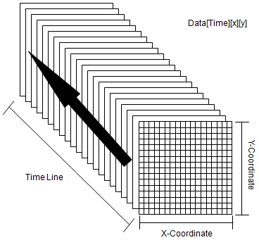
Fig. 1: Data[Time][X][y] pic credit

---

5. General Principles for Structuring Input Data

How to Determine the Input Data Structure?

The input data structure depends on the problem and the model configuration:

• Time Steps (n_steps): The length of the historical data sequence used for predictions.
• Features: Number of features available at each time step.
• Target (Y): Number of future steps you want the model to predict.

For example:

• For a task predicting 1-step-ahead: Input could be (Batch, n_steps, Features) and target could be (Batch, 1).
• For multi-step forecasting (e.g., 24 steps): Input remains (Batch, n_steps, Features) but target expands to (Batch, 24) (or (Batch, n_steps, 24) if predicting for every time step).

---

6. Predicting Outputs at Specific Time Steps

Can you always take Y_pred[i][0][23]?

Yes, if your goal is to predict 24 hours ahead for the first time step (0) of each input sequence, you can always extract Y_pred[i][0][23].

If you are interested in predictions for other time steps, you can modify the indices accordingly:

• Example: Y_pred[i][5][23] would give the 24-hour-ahead prediction for the 6th time step in the sequence.

---

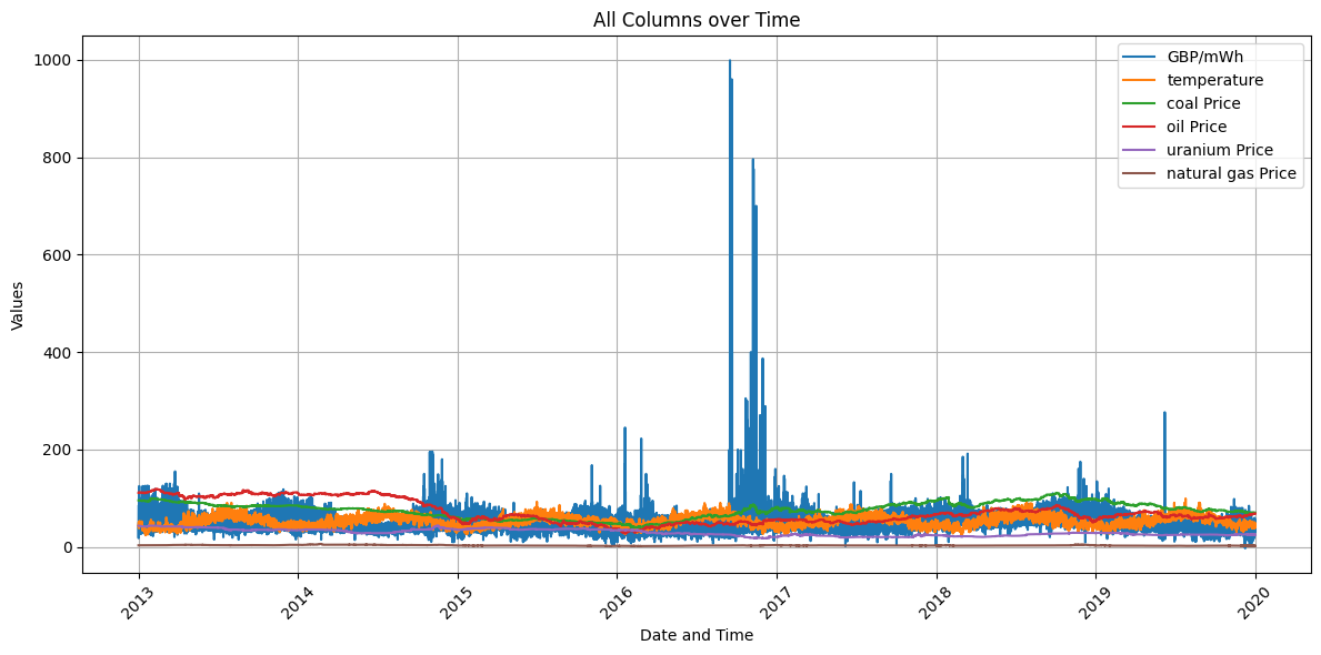
Based on the link you shared "Recurrent Neural Networks for Electricity Price Prediction":

Following code is working and applies SimpleRNN() class on data provider cleaned and shared in his Github repo:

# Import necessary libraries
import pandas as pd  
import numpy as np  
import tensorflow as tf  
from tensorflow import keras  
from matplotlib import pyplot as plt 

# Load the dataset
# Replace the file path with the one you download from the GitHub repository.
# Step 1: Load the dataset
# Read the data for the parameters from the GitHub URL into a Pandas DataFrame
url = "https://raw.githubusercontent.com/Carterbouley/ElectricityPricePrediction/refs/heads/master/re_fixed_multivariate_timeseires.csv"

# Fetch and load the CSV data
df = pd.read_csv(url, sep=",", low_memory=False)
print(df.columns) #['datetime', 'GBP/mWh', 'temperature', 'coal Price', 'oil Price', 'uranium Price','natural gas Price']

# Drop the 'datetime' column since it's not needed for the forecasting
del df['datetime']

# Convert the dataframe to a NumPy array for easier processing
data = df.values

# Define the number of past time steps used for forecasting
n_steps = 168  # One week's worth of hourly data (7 days * 24 hours)

# Reshape the data to create sequences for time series forecasting
# Each sequence includes `n_steps + 24` steps (past data + future target)
series_reshaped = np.array([
    data[i:i + (n_steps + 24)].copy()
    for i in range(len(data) - (n_steps + 24))
])
print(series_reshaped.shape)    #(61134, 192, 6)

# Split the sequences into training, validation, and test datasets
X_train = series_reshaped[:43800,      :n_steps]       # First 43800 samples for training
X_valid = series_reshaped[43800:52560, :n_steps]       # Next 8760 samples for validation
X_test  = series_reshaped[52560:,      :n_steps]       # Remaining samples for testing

# Create the target variable `Y` for forecasting
# Target consists of 24 future steps for each sequence
Y = np.empty((series_reshaped.shape[0], n_steps, 24))  # Pre-allocate target array

for step_ahead in range(1, 24 + 1):                    # Loop over each future step
    # Shift the target by `step_ahead` to align it with the input sequence
    Y[..., step_ahead - 1] = series_reshaped[..., step_ahead:step_ahead + n_steps, 0]

# Split the target variable into training, validation, and test sets
Y_train = Y[:43800]       # Training target
Y_valid = Y[43800:52560]  # Validation target
Y_test  = Y[52560:]       # Testing target

# Set random seeds for reproducibility
np.random.seed(42)
tf.random.set_seed(42)

# Define the model architecture
model6 = keras.models.Sequential([
    keras.layers.SimpleRNN(20, return_sequences=True, input_shape=[None, 6]),  # First RNN layer
    keras.layers.SimpleRNN(20, return_sequences=True),                         # Second RNN layer
    keras.layers.TimeDistributed(keras.layers.Dense(24))                       # Dense layer applied at each time step
])

# Compile the model with appropriate loss function and optimizer
model6.compile(
    loss="mean_squared_error",                  # Mean squared error loss for regression tasks
    optimizer="adam",                           # Adam optimizer for efficient training
    metrics=['mean_absolute_percentage_error']  # Evaluation metric
)

# Train the model on the training data
history = model6.fit(
    X_train, Y_train,                   # Training input and target
    epochs=10,                          # Number of epochs
    batch_size=64,                      # Batch size
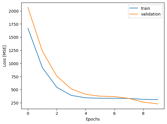
    validation_data=(X_valid, Y_valid)  # Validation data
)

print(model6.summary())
#Model: "sequential"
#┏━━━━━━━━━━━━━━━━━━━━━━━━━━━━━━━━━━━━━━┳━━━━━━━━━━━━━━━━━━━━━━━━━━━━━┳━━━━━━━━━━━━━━━━━┓
#┃ Layer (type)                         ┃ Output Shape                ┃         Param # ┃
#┡━━━━━━━━━━━━━━━━━━━━━━━━━━━━━━━━━━━━━━╇━━━━━━━━━━━━━━━━━━━━━━━━━━━━━╇━━━━━━━━━━━━━━━━━┩
#│ simple_rnn (SimpleRNN)               │ (None, None, 20)            │             540 │
#├──────────────────────────────────────┼─────────────────────────────┼─────────────────┤
#│ simple_rnn_1 (SimpleRNN)             │ (None, None, 20)            │             820 │
#├──────────────────────────────────────┼─────────────────────────────┼─────────────────┤
#│ time_distributed (TimeDistributed)   │ (None, None, 24)            │             504 │
#└──────────────────────────────────────┴─────────────────────────────┴─────────────────┘
# Total params: 5,594 (21.86 KB)
# Trainable params: 1,864 (7.28 KB)
# Non-trainable params: 0 (0.00 B)
# Optimizer params: 3,730 (14.57 KB)