Return to Revisions

I'm late for this post. Let's break down the problem into manageable parts and address each question. I'll provide insights into the format, syntax, and logic of your code.

1. Format Question: Understanding Dimensions

Why is Y_train shaped (43800, 168, 24) and not (43800, 1008, 24)?

The confusion arises from a misunderstanding of how the input data (X_train) and target labels (Y_train) are structured. Here's the breakdown:

• input data X_train (43800, 168, 6):

  Each sample in the batch (43800 timeslots) consists of 168 time steps (n_steps) of historical data. For each of these time steps, 6 features (e.g., temperature, wind speed, etc.) are provided.

• target labels Y_train (43800, 168, 24):

  Here, the second dimension (168) aligns with the 168 time steps of X_train. For each of these 168 time steps, we predict 24 future values (for each time step, we aim to forecast the next 24 hours).

  The key point is that the RNN is configured to predict 24 future steps for each of the 168 input time steps. This explains why Y_train has the shape (43800, 168, 24).

If we wanted the model to predict only 24 future values for the entire 168-step input sequence (rather than for each time step within the sequence), then Y_train would have been (43800, 24).

2. Syntax Question: Code Analysis

for step_ahead in range(1, 24 + 1):
   Y[..., step_ahead - 1] = series_reshaped[..., step_ahead:step_ahead + n_steps, 0]

Let's break it down step-by-step:

• range(1, 24 + 1):

  • Loops from 1 to 24 (inclusive), where each value represents the future step to predict (e.g., 1 hour ahead, 2 hours ahead, ..., 24 hours ahead).

• series_reshaped[..., step_ahead:step_ahead + n_steps, 0]: This slices the series_reshaped array:

  • step_ahead determines the starting point of the slice.
  • step_ahead + n_steps defines the endpoint of the slice (168 steps ahead).
  • 0 selects the feature at index 0 (assumed to be the target variable, e.g., electricity price).

• Y[..., step_ahead - 1] assigns the sliced data to the correct position in the Y array:

  • step_ahead - 1 ensures that each prediction (1-hour ahead, 2-hours ahead, etc.) is stored in a separate "slot" along the last dimension of Y.

How does this create Y with the correct dimensions (61134, 168, 24)?

The outermost loop iterates over the 24 future steps, filling the last dimension of Y one step at a time. For each future step, 168 time steps of historical data are used to generate the prediction.

• Predicting Future Values

Why do we use Y_pred[i][0][23] in the prediction code?

Y_pred = model6.predict(X_test)
last_list = []
for i in range(len(Y_pred)):
    last_list.append(Y_pred[i][0][23])

• Y_pred[i][0][23]:
  • i: Refers to the i-th sample in the batch of predictions.
  • 0: Refers to the first time step within the sequence (the initial context for prediction).
  • 23: Selects the 24th prediction (corresponding to 24 hours ahead).

This selection makes sense because you are interested in the 24-hour-ahead prediction for the first time step of each input sequence.

4. Why is Y shaped (Batch, 168, 24) instead of (Batch, 24)?

This is because the RNN is configured with return_sequences=True. Here’s what it means:

• return_sequences=True: The RNN outputs a prediction for every time step in the input sequence (168 steps).
• For each of these 168 steps, the model predicts the next 24 steps into the future, resulting in a target shape of (Batch, 168, 24).

If the model was configured with return_sequences=False, it would only produce a single prediction for the entire input sequence (likely (Batch, 24)).

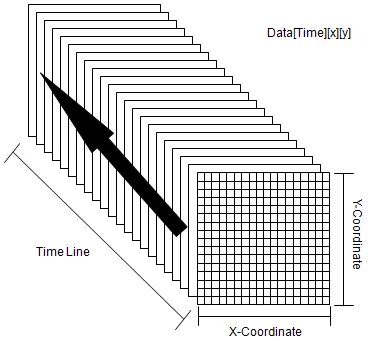
Fig. 1: Data[Time][X][y] pic credit

5. General Principles for Structuring Input Data

How to Determine the Input Data Structure?

The input data structure depends on the problem and the model configuration:

• Time Steps (n_steps): The length of the historical data sequence used for predictions.
• Features: Number of features available at each time step.
• Target (Y): Number of future steps you want the model to predict.

For example:

• For a task predicting 1-step-ahead: Input could be (Batch, n_steps, Features) and target could be (Batch, 1).
• For multi-step forecasting (e.g., 24 steps): Input remains (Batch, n_steps, Features) but target expands to (Batch, 24) (or (Batch, n_steps, 24) if predicting for every time step).

6. Predicting Outputs at Specific Time Steps

Can you always take Y_pred[i][0][23]?

Yes, if your goal is to predict 24 hours ahead for the first time step (0) of each input sequence, you can always extract Y_pred[i][0][23].

If you are interested in predictions for other time steps, you can modify the indices accordingly:

• Example: Y_pred[i][5][23] would give the 24-hour-ahead prediction for the 6th time step in the sequence.

Based on the link you shared "Recurrent Neural Networks for Electricity Price Prediction":

Following code is working and applies SimpleRNN() class on data provider cleaned and shared in his Github repo:

# Import necessary libraries
import pandas as pd  
import numpy as np  
import tensorflow as tf  
from tensorflow import keras  
from matplotlib import pyplot as plt 

# Load the dataset
# Replace the file path with the one you download from the GitHub repository.
# Step 1: Load the dataset
# Read the data for the parameters from the GitHub URL into a Pandas DataFrame
url = "https://raw.githubusercontent.com/Carterbouley/ElectricityPricePrediction/refs/heads/master/re_fixed_multivariate_timeseires.csv"

# Fetch and load the CSV data
df = pd.read_csv(url, sep=",", low_memory=False)
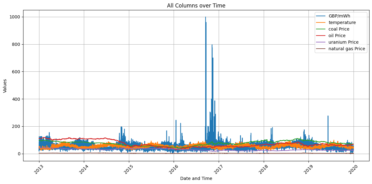
print(df.columns) #['datetime', 'GBP/mWh', 'temperature', 'coal Price', 'oil Price', 'uranium Price','natural gas Price']

# Drop the 'datetime' column since it's not needed for the forecasting
del df['datetime']

# Convert the dataframe to a NumPy array for easier processing
data = df.values

# Define the number of past time steps used for forecasting
n_steps = 168  # One week's worth of hourly data (7 days * 24 hours)

# Reshape the data to create sequences for time series forecasting
# Each sequence includes `n_steps + 24` steps (past data + future target)
series_reshaped = np.array([
    data[i:i + (n_steps + 24)].copy()
    for i in range(len(data) - (n_steps + 24))
])
print(series_reshaped.shape)    #(61134, 192, 6)

# Split the sequences into training, validation, and test datasets
X_train = series_reshaped[:43800,      :n_steps]       # First 43800 samples for training
X_valid = series_reshaped[43800:52560, :n_steps]       # Next 8760 samples for validation
X_test  = series_reshaped[52560:,      :n_steps]       # Remaining samples for testing

# Create the target variable `Y` for forecasting
# Target consists of 24 future steps for each sequence
Y = np.empty((series_reshaped.shape[0], n_steps, 24))  # Pre-allocate target array

for step_ahead in range(1, 24 + 1):                    # Loop over each future step
    # Shift the target by `step_ahead` to align it with the input sequence
    Y[..., step_ahead - 1] = series_reshaped[..., step_ahead:step_ahead + n_steps, 0]

# Split the target variable into training, validation, and test sets
Y_train = Y[:43800]       # Training target
Y_valid = Y[43800:52560]  # Validation target
Y_test  = Y[52560:]       # Testing target

# Set random seeds for reproducibility
np.random.seed(42)
tf.random.set_seed(42)

# Define the model architecture
model6 = keras.models.Sequential([
    keras.layers.SimpleRNN(20, return_sequences=True, input_shape=[None, 6]),  # First RNN layer
    keras.layers.SimpleRNN(20, return_sequences=True),                         # Second RNN layer
    keras.layers.TimeDistributed(keras.layers.Dense(24))                       # Dense layer applied at each time step
])

# Compile the model with appropriate loss function and optimizer
model6.compile(
    loss="mean_squared_error",                  # Mean squared error loss for regression tasks
    optimizer="adam",                           # Adam optimizer for efficient training
    metrics=['mean_absolute_percentage_error']  # Evaluation metric
)

# Train the model on the training data
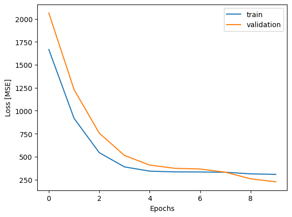
history = model6.fit(
    X_train, Y_train,                   # Training input and target
    epochs=10,                          # Number of epochs
    batch_size=64,                      # Batch size
    validation_data=(X_valid, Y_valid)  # Validation data
)

print(model6.summary())
#Model: "sequential"
#┏━━━━━━━━━━━━━━━━━━━━━━━━━━━━━━━━━━━━━━┳━━━━━━━━━━━━━━━━━━━━━━━━━━━━━┳━━━━━━━━━━━━━━━━━┓
#┃ Layer (type)                         ┃ Output Shape                ┃         Param # ┃
#┡━━━━━━━━━━━━━━━━━━━━━━━━━━━━━━━━━━━━━━╇━━━━━━━━━━━━━━━━━━━━━━━━━━━━━╇━━━━━━━━━━━━━━━━━┩
#│ simple_rnn (SimpleRNN)               │ (None, None, 20)            │             540 │
#├──────────────────────────────────────┼─────────────────────────────┼─────────────────┤
#│ simple_rnn_1 (SimpleRNN)             │ (None, None, 20)            │             820 │
#├──────────────────────────────────────┼─────────────────────────────┼─────────────────┤
#│ time_distributed (TimeDistributed)   │ (None, None, 24)            │             504 │
#└──────────────────────────────────────┴─────────────────────────────┴─────────────────┘
# Total params: 5,594 (21.86 KB)
# Trainable params: 1,864 (7.28 KB)
# Non-trainable params: 0 (0.00 B)
# Optimizer params: 3,730 (14.57 KB)