MAD vs RMSE vs MAE vs MSLE vs R²: When to use which?

Question

In regression problems, you can use various different metrics to check how well your model is doing:

• Mean Absolute Deviation (MAD): In $[0, \infty)$, the smaller the better
• Root Mean Squared Error (RMSE): In $[0, \infty)$, the smaller the better
• Median Absolute Error (MAE): In $[0, \infty)$, the smaller the better
• Mean Squared Log Error (MSLE): In $[0, \infty)$, the smaller the better
• R², coefficient of determination: In $(-\infty, 1]$ not necessarily the bigger the better

Are there any strong reasons not to use one or the other?

Answer 1

Well actually these can give you different insights into your models errors. If $y$ is your target, $p$ your prediction and $e = p - y$ the errors:

• Mean Error: $ME = mean(e)$
  

In (-∞,∞), the closer to 0 the better.
Measures additive bias in the error. Unbiased estimates should have the same mean as your target thus ME should be close to 0, if it's positive your predictions overestimate the target, if it's negative they underestimate.

• Root Mean Squared Error: $RMSE = \sqrt{mean(e^2)}$.
  

In [0,∞), the smaller the better.
Measures the mean square magnitude of errors. Root square is taken to make the units of the error be the same as the units of the target. This measure gives more weight to large deviations such as outliers, since large differences squared become larger and small (smaller than 1) differences squared become smaller.

• Mean Absolute Error: $MAE = mean(|e|)$.
  

In [0,∞), the smaller the better.
Measures the absolute magnitude of errors and it's units are the same as the units of the target. Makes for more easily interprectable errors and gives less weight to outliers. However a model with good $MAE$ can have punctually very high errors.

• (Root) Mean Squared Log Error: $MSLE= mean((log(p+1)-log(y+1))^2)$.
  

In [0,∞), the smaller the better.
This is useful when dealing with right skewed targets, since taking the log transform makes the target more normally distributed. In practice it's usually achieved by changing the target to $\hat{y}=log(y+1)$ and then predicting as $y=e^\hat{y}-1$

• Median Absolute Deviation: $MAD = median(e - median(e))$.
  

In [0,∞), the smaller the better.
This is a spread metric similar to standard deviation but meant to be more robust to outliers. Instead of taking means of squares as the sd, MAD takes medians of absolutes making it more robust.

• R², coefficient of determination:
  

In (−∞,1] the closer to 1 the better Is a measure of the ratio of variability that your model can capture vs the natural variability in the target variable.

In practice I usually use a combination of $ME$, $R^2$ and: $RMSE$ if there are no outliers in the data, $MAE$ if I have a large dataset and there may be outliers, $RMLSE$ if the target is right skewed.

This link offers a very nice overview on the matter: http://www.cawcr.gov.au/projects/verification/#Methods_for_foreasts_of_continuous_variables

Answer 2

I recommend that you change your point of view a bit: first decide on what forecast you want, then choose an appropriate error measure.

Let me explain.

Suppose we are not directly predicting a single value, but an entire (predictive) density $\hat{F}$ for our future unknown outcome, which we then want to summarize or condense into a single number. Assuming that the predictive density is a correct summary of the distribution of the outcome we are predicting, we can now ask which "one-number summary" yields the lowest expected error for our chosen error measure.

And here, we should keep in mind that different error measures are minimized in expectation by different one-number summaries.

• The MSE and RMSE is minimized by the expectation of $\hat{F}$. Showing this is a rather simple and fun calculus exercise. So is $1-R^2$ (let's work with minimizing this rather than maximizing $R^2$, which is of course the same, but makes life easier), since $R^2$ is just a reformulation of MSE.
• The expected absolute error, your MAD, is minimized by the median of $\hat{F}$.
• The hinge or quantile loss is minimized by the appropriate quantile of $\hat{F}$, which is of course exactly why we use it in quantile regression, or in any way of predicting conditional quantiles.

Thus, if we want conditional median predictions, we should use the MAD, and if we want conditional expectations, we should use the (R)MSE. (This is a reformulation of the common meme that "the MAD is less affected by outliers than the MSE", and the discussion above illustrates why I believe this is a mistaken way of looking at things.) If we want our model to yield expectation forecasts, using the MAD may give the misleading impression that we are not doing a good job. The difference of course depends on how asymmetric our conditional density is.

Now, you might argue that we do not care about predictive densities, we only want single-number predictions. To which I would answer that even if we are not interested in densities, they are still very much interested in us. As long as we are dealing with noisy data, (error) distributions are still very relevant. Even if we never explicitly consider predictive densities, using the (R)MSE will reward predictions that are close to the conditional expectation, and the MAD will reward ones that are close to the conditional median, simply because calculating them deals with the distribution of the actuals on which we evaluate our predictions.

And this is where my recommendation comes from: we should first decide on which "one number summary" ("functional") of the unknown future distribution we want (expectation, median, quantile), and then pick the error measure that elicits that functional (MSE, MAD, pinball loss).

Kolassa (2020), a commentary on the M4 forecasting competition, makes the point in somewhat more detail. And here I discuss the Mean Absolute Percentage Error (MAPE) in the same way: What are the shortcomings of the Mean Absolute Percentage Error (MAPE)?

---

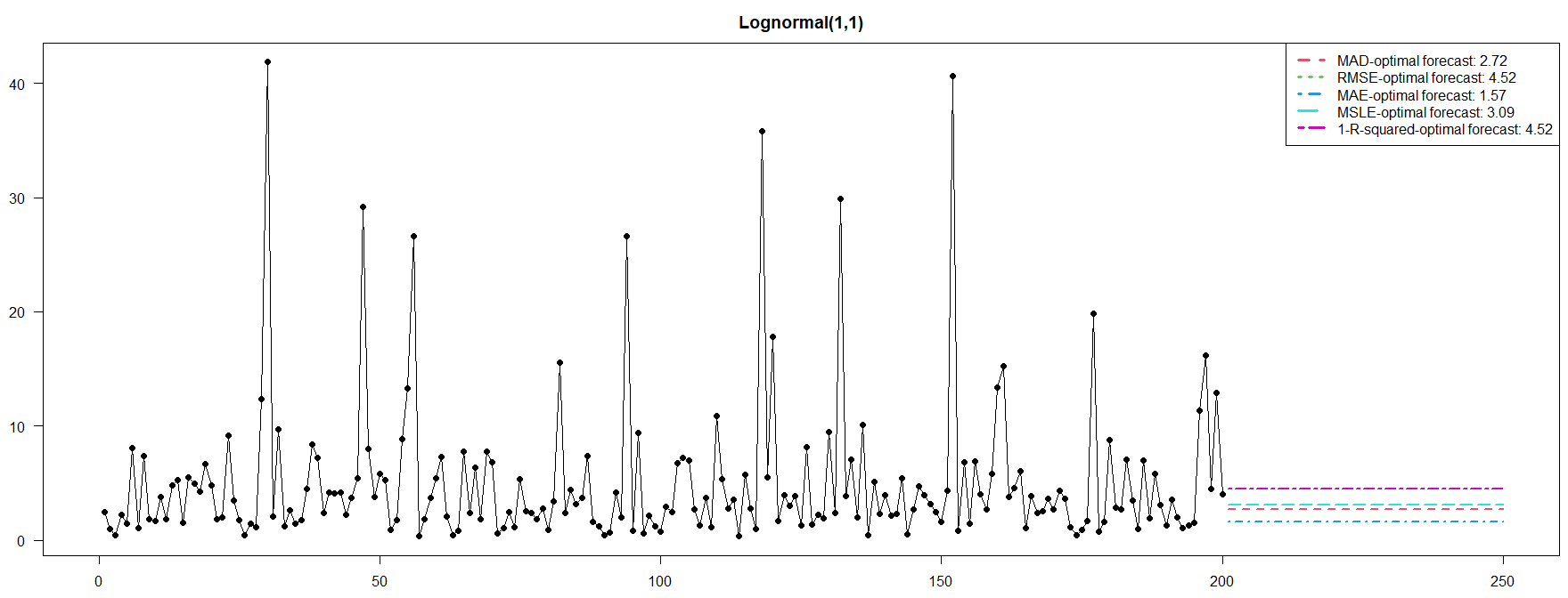
As an example, assume that conditional on our model and predictors, we believe that the future realization follows a lognormal distribution with log-mean $\mu=1$ and log-variance $\sigma^2=1$. Below is a simulated example in time series format, together with the point predictions that minimize each expected error, based on $10^5$ simulations. Since the simulations are IID, the optimal point predictions will be a horizontal flat line. Note that minimizing the MAD, the MAE or the MSLE leads to predictions that are far below the expectation of $\exp\big(\mu+\frac{\sigma^2}{2}\big)=\exp 1.5\approx 4.48$. (I hesitate to call them "biased", because per above, these error measures elicit exactly what they are eliciting, and the issue is just that this elicited functional is not the expectation.)

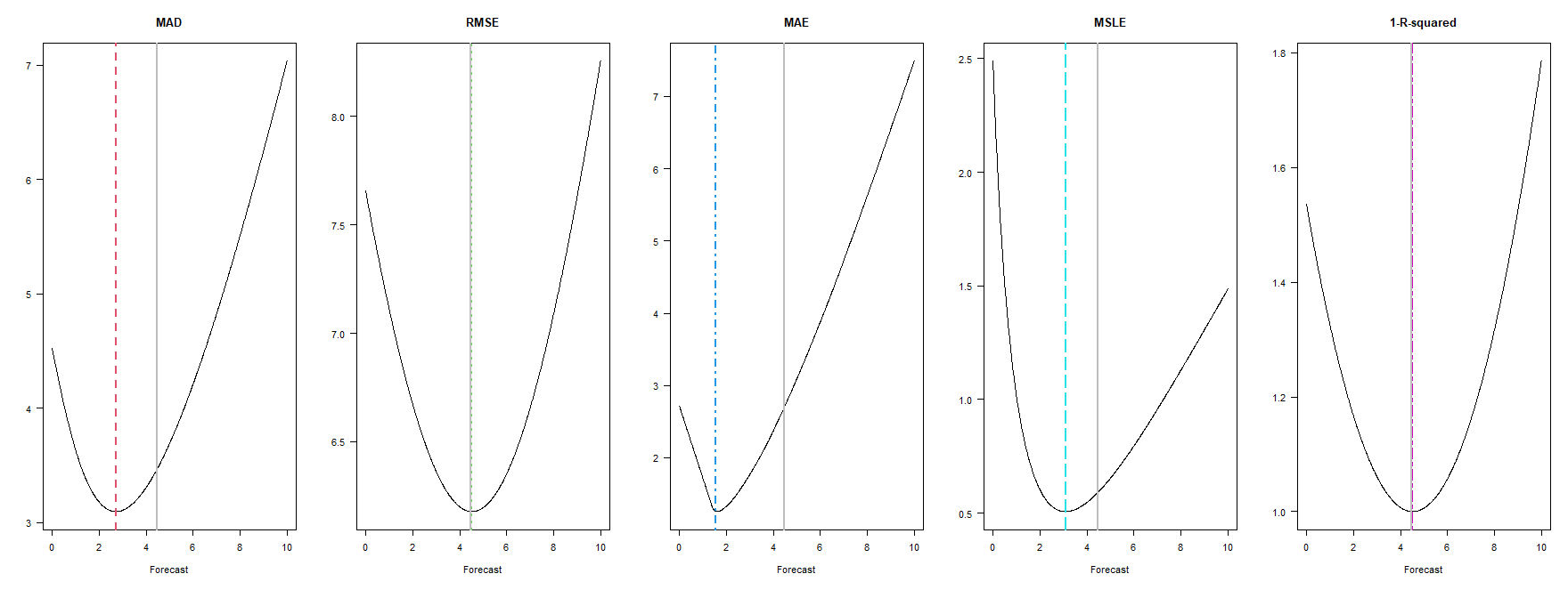
Actually, we can look at different predictions and calculate the expected errors over our $10^5$ simulations. We can then deduce which prediction minimizes the expected error. See below for these plots - the colored vertical lines in each case give the optimal predictions (and correspond to the horizontal prediction lines above, because that is how I got them), while the vertical grey line gives the expectation at about 4.48.

---

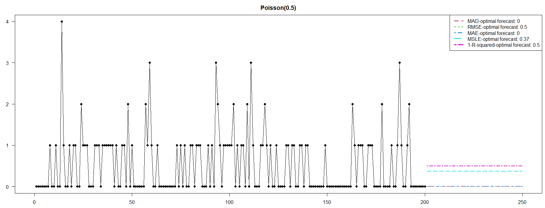
For a second example, we can simulate Poisson data with mean and variance $\lambda=0.5$:

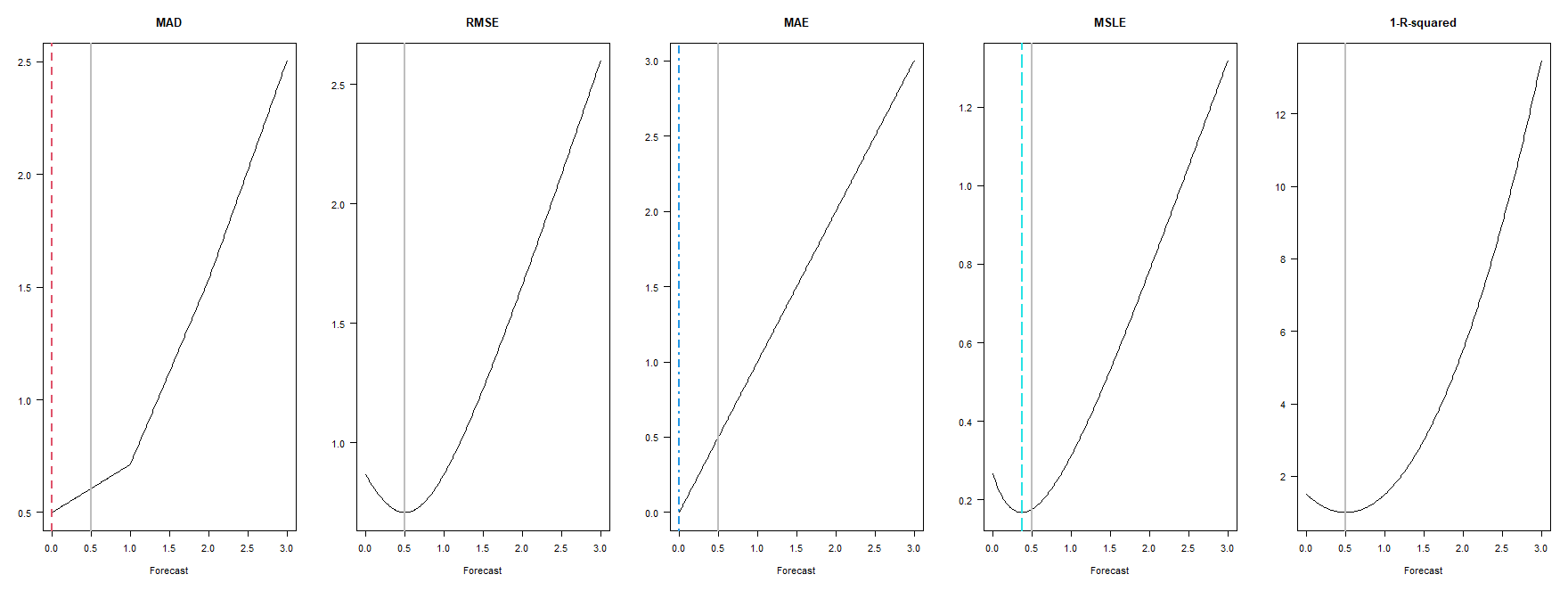
Fun fact: trying to minimize the MAD or MAE incentivizes us to output a flat zero forecast. This is exactly as it should be, since the median of a Poisson(0.5) is zero, but it did make some people working in intermittent demand forecasting rather nervous (Kolassa, 2016). Here are the expected errors against candidate predictions:

---

R code for the plots:

plot_result <- function(fcsts,errors,error_name,col,lty,expectation) {
    plot(fcsts,errors,main=error_name,type="l",xlab="Forecast",ylab="")
    abline(v=fcsts[which.min(errors)],col=col,lwd=2,lty=lty)
    abline(v=expectation,col="grey",lwd=2)
}

calculate_errors <- function(fcsts,sims) {
    errors <- list()
    errors[["MAD"]] <- sapply(fcsts,function(xx)mean(abs(xx-sims)))
    errors[["RMSE"]] <- sapply(fcsts,function(xx)sqrt(mean((xx-sims)^2)))
    errors[["MAE"]] <- sapply(fcsts,function(xx)median(abs(xx-sims)))
    errors[["MSLE"]] <- sapply(fcsts,function(xx)mean((log(xx+1)-log(sims+1))^2))
    errors[["1-R-squared"]] <-
        1-sapply(fcsts,function(xx)1-mean((xx-sims)^2)/(mean((sims-mean(sims))^2)))
    errors
}

#############################################################
# lognormal example
#############################################################

set.seed(2023)
mm <- 1
ss.sq <- 1
sims <- rlnorm(1e5,meanlog=mm,sdlog=sqrt(ss.sq))
fcsts <- seq(0,10,by=.01)
errors <- calculate_errors(fcsts,sims)

opar <- par(mai=c(.5,.5,.5,.1),las=1)
    plot(sims[1:200],type="o",pch=19,xlab="",ylab="",
        main=paste0("Lognormal(",mm,",",ss.sq,")"),
        xlim=c(0,250))
    for ( ii in seq_along(errors) ) {
        lines(c(201,250),rep(fcsts[which.min(errors[[ii]])],2),
            lty=ii+1,col=ii+1,lwd=2)
    }
    legend("topright",col=seq_along(errors)+1,lty=seq_along(errors)+1,lwd=3,
        legend=paste0(names(errors),"-optimal forecast: ",
            round(fcsts[sapply(errors,which.min)],2)))
par(opar)

opar <- par(mfrow=c(1,length(errors)),las=1,mai=c(.8,.5,.5,.2))
    for ( ii in seq_along(errors) ) {
        plot_result(fcsts,errors[[ii]],error_name=names(errors)[[ii]],
            col=ii+1,lty=ii+1,expectation=exp(mm+ss.sq/2))
    }
par(opar)


#############################################################
# Poisson example
#############################################################

set.seed(2023)
lambda <- 0.5
sims <- rpois(1e6,lambda=lambda)
fcsts <- seq(0,3,by=.01)
errors <- calculate_errors(fcsts,sims)

opar <- par(mai=c(.5,.5,.5,.1),las=1)
    plot(sims[1:200],type="o",pch=19,xlab="",ylab="",
        main=paste0("Poisson(",lambda,")"),
        xlim=c(0,250))
    for ( ii in seq_along(errors) ) {
        lines(c(201,250),rep(fcsts[which.min(errors[[ii]])],2),
            lty=ii+1,col=ii+1,lwd=2)
    }
    legend("topright",col=seq_along(errors)+1,lty=seq_along(errors)+1,lwd=3,
        legend=paste0(names(errors),"-optimal forecast: ",
            round(fcsts[sapply(errors,which.min)],2)))
par(opar)

opar <- par(mfrow=c(1,length(errors)),las=1,mai=c(.8,.5,.5,.2))
    for ( ii in seq_along(errors) ) {
        plot_result(fcsts,errors[[ii]],error_name=names(errors)[[ii]],
            col=ii+1,lty=ii+1,expectation=lambda)
    }
par(opar)

Answer 3

I have very rough ideas for some:

• MAD if a deviation of 2 is "double as bad" than having a deviation of 1.
• RMSE if the value deteriorates more quickly - punishes outliers hard! (can be good or bad)
• MAE if I'm not interested in complete outliers, but only in "typical" cases (as I usually fence the outputs to a reasonable range, this is almost the same as MAD)

For MSLE and R², I have no idea when it is better suited than the others.