How to numerically estimate MLE estimators in python when gradients are very small far from the optimal solution?

Question

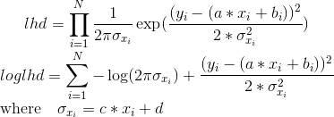
I am exploring how to model a data set using normal distributions with both mean and variance defined as linear functions of independent variables.

Something like N ~ (f(x), g(x)).

I generate a random sample like this:

def draw(x):
    return norm(5 * x + 2, 3 *x + 4).rvs(1)[0]

So I want to retrieve 5, 2 and 4 as the parameters for my distribution.

I generate my sample:

smp = np.zeros((100,2))

for i in range(0, len(smp)):
    smp[i][0] = i
    smp[i][1] = draw(i)

The likelihood function is:

def lh(p):
    p_loc_b0 = p[0]
    p_loc_b1 = p[1]
    p_scl_b0 = p[2]
    p_scl_b1 = p[3]

    l = 1
    for i in range(0, len(smp)):
        x = smp[i][0]
        y = smp[i][1]
        l = l * norm(p_loc_b0 + p_loc_b1 * x, p_scl_b0 + p_scl_b1 * x).pdf(y)

    return -l

So the parameters for the linear functions used in the model are given in the p 4-variable vector.

Using scipy.optimize, I can solve for the MLE parameters using an extremely low xtol, and already giving the solution as the starting point:

fmin(lh, x0=[2,5,3,4], xtol=1e-35)

Which does not work to well:

Warning: Maximum number of function evaluations has been exceeded.
array([ 3.27491346,  4.69237042,  5.70317719,  3.30395462])

Raising the xtol to higher values does no good.

So i try using a starting solution far from the real solution:

>>> fmin(lh, x0=[1,1,1,1], xtol=1e-8)
Optimization terminated successfully.
         Current function value: -0.000000
         Iterations: 24
         Function evaluations: 143
array([ 1.,  1.,  1.,  1.])

Which makes me think:

PDF are largely clustered around the mean, and have very low gradients only a few standard deviations away from the mean, which must be not too good for numerical methods.

So how does one go about doing these kind of numerical estimation in functions where gradient is very near to zero away from the solution?

Answer 1

There are several reasons why you are getting erroneous results. First, you should consider using log likelihood instead of likelihood. There are numerical issues with multiplying many small numbers(imagine if you had millions of samples you had to multiply millions of small numbers for the lhd). Also taking gradients for optimization methods that require gradients is often easier when you are dealing with the log likelihood. In general, it is good to have an objective which is a sum rather than a product of variables when dealing with optimization problems.

Second, fmin is using Nelder-Mead simplex algorithm which has no convergence guarantees according to scipy documentation. This means the convergence is totally random and you should not expect to find parameters close to the originals. To get around this, I would suggest you to use a gradient based method like stochastic gradient descent or BFGS. Since you know the generative model (rvs are Gaussian distributed) you can write the likelihood and log likelihood as:

Where a,b,c and d are your model parameters 5,2,3 and 4 respectively. Then take the gradient with respect to [a,b,c,d] and feed that into prime input of fmin_bfgs. Note that due to varying variance what could be solved by just linear regression is now a nastier problem.

Finally, you may also want to check Generalized least squares here and here, which talk about your problem and offer several available solutions.

Good luck!