3
$\begingroup$

This is how I understand the perceptron algorithm.

The perceptron loss function is the hinge loss $\ell(w,x,y) = \max(0, -yw\cdot x)$. Suppose the data set is $D = \{(x_1,y_1),\dots,(x_n,y_n)\}$ with $y_i \in \{-1,1\}$. The perceptron criterion is $$ E(w) = \sum_i \ell(w, x_i, y_i) = \sum_i \max(0, -y_iw\cdot x). $$ The perceptron algorithm tries to minimize $E(w)$ using gradient descent. The gradient of $E(w)$ with respect to $w$ is $$ \nabla E(w) = \sum_i \left\{ \begin{array}{ll} \mathbf{0} & \text{ if } \ell(w,x_i,y_i) = 0\\ -y_ix_i & \text{ otherwise } \end{array}\right.. $$ So the perceptron updates the $w$ according to $$ w^{(t+1)} = w^{(t)} - \eta \nabla E(w^{(t)}) = w^{(t)} + \eta \sum_{i\in M(t)} y_ix_i $$ where $M(t)$ is the set of points misclassified by $w^{(t)}$. Since we can define another equivalent sequence of weight vectors $v^{(t)} = (1/\eta)w^{(t)}$, we can just take $\eta = 1$.

I know that $w^{(t)}$ will converge to a seperating hyperplane if one exists and $E(w)$ will converge to $0$.

My question is about when the data set is not linearly separable. In that case, does $E(w)$ converge to some minimum?

If $E(w)$ attains some minimum, its gradient there has to be $\mathbf{0}$. One possibility is that all the terms in the sum of $\nabla E$ are 0, which means that the dataset is linearly seperable and this is contradiction. The other possibility is that the sum of $-y_ix_i$ over the misclassified points is somehow $\mathbf{0}$.

$\endgroup$

2 Answers 2

2
$\begingroup$

The behavior appears to actually depend on the learning rate $\eta$; a smaller $\eta$ affects which points are misclassified in the next iteration, which affects the weight update more than just by the simple scaling you alluded to.

With appropriately small learning rates though, it seems you are guaranteed convergence to some local minimum, if you avoid certain degenerate situations that would give e.g. a constant loss surface. Exactly what you describe happens at these minima: the loss to the misclassified points of either class equal each other.

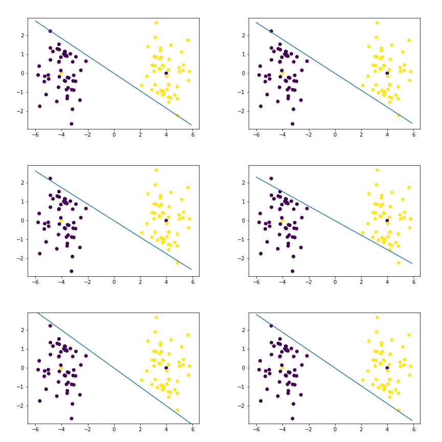
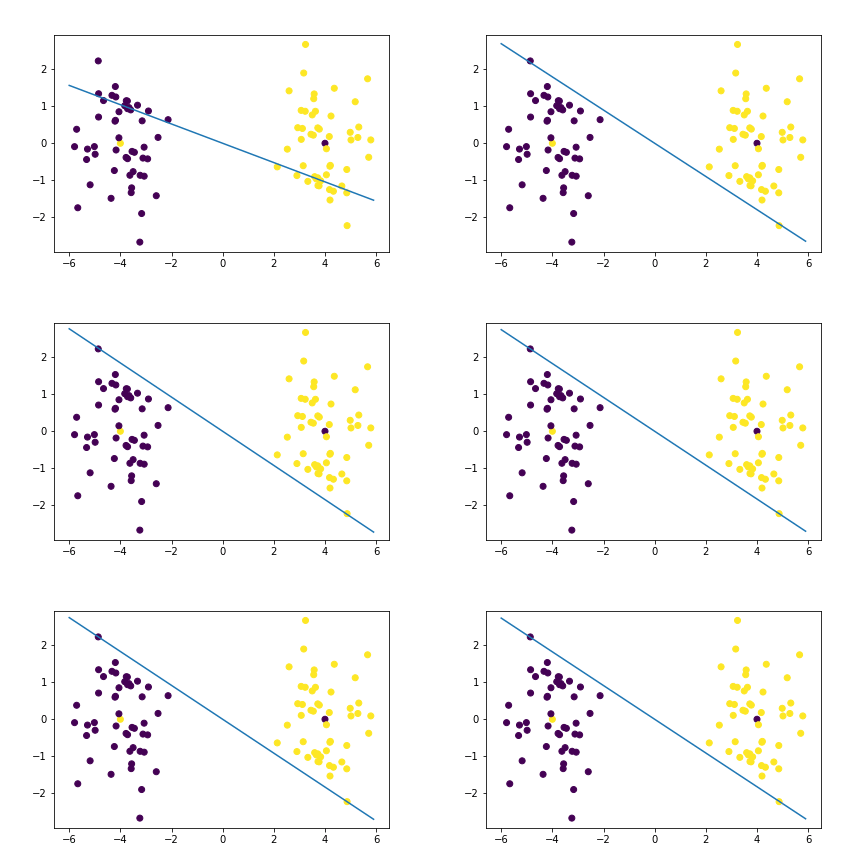
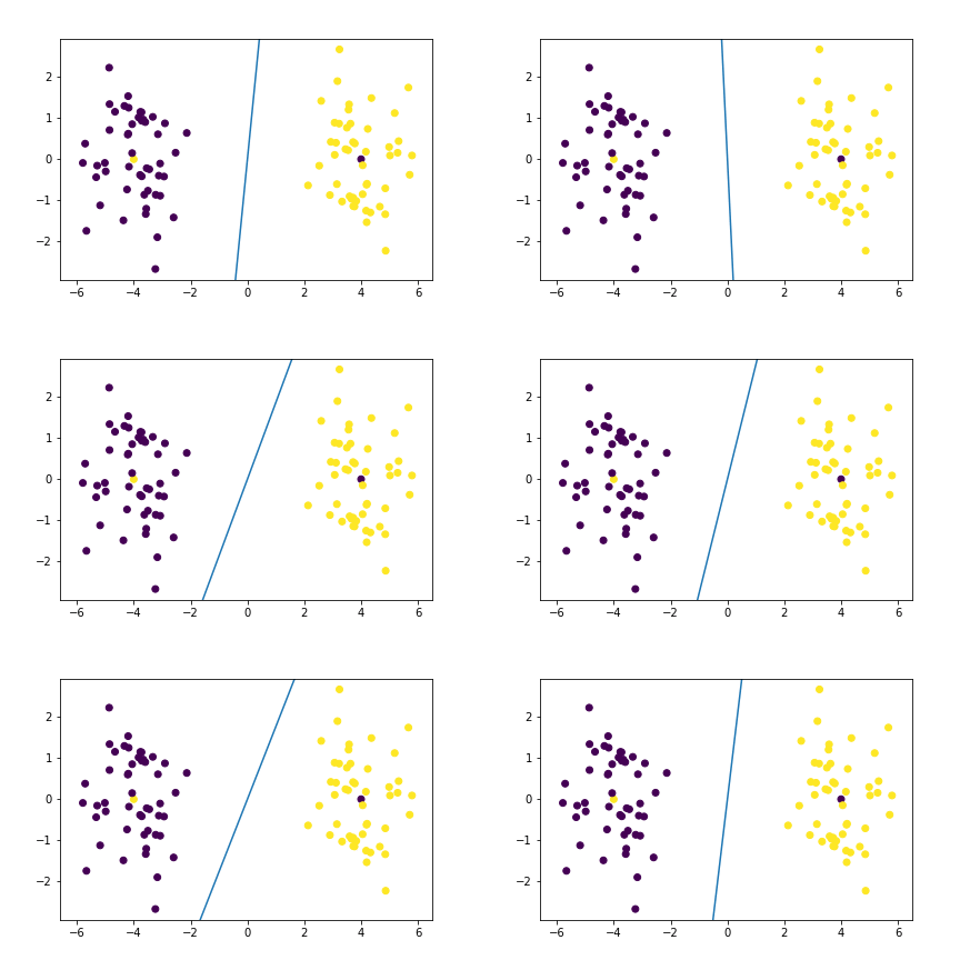
I put together a short demonstration in this colab notebook (github link). Below are some animations of the evolution of the decision line during the gradient descent, starting at the top with a large learning rate and decreasing it from there. In this situation, there should be two local minima, the two "tangents" to the "blobs" (possibly pulled in a little, misclassifying a couple of extra points if it can decrease the loss on the central points a little more than the cost for the newly misclassified points).

with large learning rate, decision boundary fluctuates quite a lot

with smaller learning rate, decision boundary converges a bit better

with even smaller learning rate, convergence is slower but much more stable

$\endgroup$
-1
$\begingroup$

Let $\{(x_j, y_j)\}_{j\in J}$ be the set of points misclassified by $w$ (the ones with non-zero terms in the sum of $\nabla E$). Under the hypothesis that $-\sum_{j\in J} y_j x_j = 0$,

$$\sum_{j\in J} y_j w \cdot x_j = w \cdot \left(\sum_{j\in J} y_j x_j\right) = 0,$$

therefore the data are linearly separable.

$\endgroup$

Your Answer

By clicking “Post Your Answer”, you agree to our terms of service and acknowledge you have read our privacy policy.

Not the answer you're looking for? Browse other questions tagged or ask your own question.