Choosing a learning rate

Question

I'm currently working on implementing Stochastic Gradient Descent, SGD, for neural nets using back-propagation, and while I understand its purpose I have some questions about how to choose values for the learning rate.

• Is the learning rate related to the shape of the error gradient, as it dictates the rate of descent?
• If so, how do you use this information to inform your decision about a value?
• If it's not what sort of values should I choose, and how should I choose them?
• It seems like you would want small values to avoid overshooting, but how do you choose one such that you don't get stuck in local minima or take to long to descend?
• Does it make sense to have a constant learning rate, or should I use some metric to alter its value as I get nearer a minimum in the gradient?

In short: How do I choose the learning rate for SGD?

Answer 1

• Is the learning rate related to the shape of the error gradient, as it dictates the rate of descent?

  • In plain SGD, the answer is no. A global learning rate is used which is indifferent to the error gradient. However, the intuition you are getting at has inspired various modifications of the SGD update rule.

• If so, how do you use this information to inform your decision about a value?

  • Adagrad is the most widely known of these and scales a global learning rate η on each dimension based on l2 norm of the history of the error gradient gt on each dimension:

    

  • Adadelta is another such training algorithm which uses both the error gradient history like adagrad and the weight update history and has the advantage of not having to set a learning rate at all.

• If it's not what sort of values should I choose, and how should I choose them?

  • Setting learning rates for plain SGD in neural nets is usually a process of starting with a sane value such as 0.01 and then doing cross-validation to find an optimal value. Typical values range over a few orders of magnitude from 0.0001 up to 1.

• It seems like you would want small values to avoid overshooting, but how do you choose one such that you don't get stuck in local minima or take too long to descend? Does it make sense to have a constant learning rate, or should I use some metric to alter its value as I get nearer a minimum in the gradient?

  • Usually, the value that's best is near the highest stable learning rate and learning rate decay/annealing (either linear or exponentially) is used over the course of training. The reason behind this is that early on there is a clear learning signal so aggressive updates encourage exploration while later on the smaller learning rates allow for more delicate exploitation of local error surface.

Answer 2

Below is a very good note (page 12) on learning rate in Neural Nets (Back Propagation) by Andrew Ng. You will find details relating to learning rate.

http://web.stanford.edu/class/cs294a/sparseAutoencoder_2011new.pdf

For your 4th point, you're right that normally one has to choose a "balanced" learning rate, that should neither overshoot nor converge too slowly. One can plot the learning rate w.r.t. the descent of the cost function to diagnose/fine tune. In practice, Andrew normally uses the L-BFGS algorithm (mentioned in page 12) to get a "good enough" learning rate.

Answer 3

Selecting a learning rate is an example of a "meta-problem" known as hyperparameter optimization. The best learning rate depends on the problem at hand, as well as on the architecture of the model being optimized, and even on the state of the model in the current optimization process! There are even software packages devoted to hyperparameter optimization such as spearmint and hyperopt (just a couple of examples, there are many others!).

Apart from full-scale hyperparameter optimization, I wanted to mention one technique that's quite common for selecting learning rates that hasn't been mentioned so far. Simulated annealing is a technique for optimizing a model whereby one starts with a large learning rate and gradually reduces the learning rate as optimization progresses. Generally you optimize your model with a large learning rate (0.1 or so), and then progressively reduce this rate, often by an order of magnitude (so to 0.01, then 0.001, 0.0001, etc.).

This can be combined with early stopping to optimize the model with one learning rate as long as progress is being made, then switch to a smaller learning rate once progress appears to slow. The larger learning rates appear to help the model locate regions of general, large-scale optima, while smaller rates help the model focus on one particular local optimum.

Answer 4

Copy-pasted from my masters thesis:

• If the loss does not decrease for several epochs, the learning rate might be too low. The optimization process might also be stuck in a local minimum.
• Loss being NAN might be due to too high learning rates. Another reason is division by zero or taking the logarithm of zero.
• Weight update tracking: Andrej Karpathy proposed in the 5th lecture of CS231n to track weight updates to check if the learning rate is well-chosen. He suggests that the weight update should be in the order of 10−3. If the weight update is too high, then the learning rate has to be decreased. If the weight update is too low, then the learning rate has to be increased.
• Typical learning rates are in [0.1, 0.00001]

Answer 5

Learning rate , transformed as "step size" during our iteration process , has been a hot issue for years , and it will go on .

There are three options for step size in my concerning :

• One is related to "time" , and each dimension shall share the same step size . You might have noticed something like

$\it\huge\bf\frac{\alpha}{\sqrt{t}}$

while t demonstrates the current iteration number , alpha is hyper parameter

• the next one is connected with gradient , and each dimension have their own step size . You might have noticed something like

$\it\huge\frac{1}{\frac{\alpha}{\beta + \sqrt{\sum_{s = 1}^{t - 1}{g_{s}^2}}} - \frac{\alpha}{\beta + \sqrt{\sum_{s = 1}^{t}{g_{s}^2}}}}$

while alpha and beta are hyper parameter , g demonstrates gradient

• the last one is the combination of time and gradient , and it should be like

$\it\huge\frac{1}{\frac{\alpha}{\beta + \sqrt{\sum_{s = 1}^{t - 1}{g_{s}^2}}} -\frac{\alpha}{\beta + \sqrt{\sum_{s = 1}^{t}{g_{s}^2}}}} + \frac{\gamma}{\sqrt{t}}$

or

$\it\huge\frac{1}{\frac{\alpha}{\beta + \sqrt{\sum_{s = 1}^{t - 1}{g_{s}^2}}} - \frac{\alpha}{\beta + \sqrt{\sum_{s = 1}^{t}{g_{s}^2}}}} * \frac{\gamma}{\sqrt{t}}$

Hopes this will help you , good luck -)

Answer 6

Adding to David's answer, in fastai is where I found the concept of finding the best learning rate for that data, using a particular architecture.

But that thing exists only on fastai/pytorch. Recently someone made a keras implementation.

which in turn are based on these papers:

• A disciplined approach to neural network hyper-parameters: Part 1 -- learning rate, batch size, momentum, and weight decay
• Super-Convergence: Very Fast Training of Residual Networks Using Large Learning Rates

Hope this helps.

Answer 7

Neural networks are often trained by gradient descent on the weights. This means at each iteration we use backpropagation to calculate the derivative of the loss function with respect to each weight and subtract it from that weight. However, if you actually try that, the weights will change far too much each iteration, which will make them “overcorrect” and the loss will actually increase/diverge. So in practice, people usually multiply each derivative by a small value called the “learning rate” before they subtract it from its corresponding weight.

You can also think of a neural networks loss function as a surface, where each direction you can move in represents the value of a weight. Gradient descent is like taking leaps in the current direction of the slope, and the learning rate is like the length of the leap you take.

Answer 8

Let me give a brief introduction to another approach on choosing the learning rate, based on Jeremy Howard's Deep Learning course 1. If you want to dig deeper, see this blogpost.

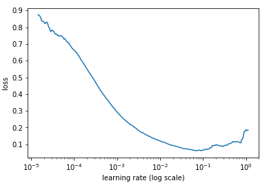
The learning rate proposed in Jeremy Howard's course is based on a systematic way to try different learning rates and choose the one that makes the loss function go down the most. This is done by feeding many batches to the mini-batch gradient descent method, and increasing the learning rate every new batch you feed to the method. When the learning rate is very small, the loss function will decrease very slowly. When the learning rate is very big, the loss function will increase. Inbetween these two regimes, there is an optimal learning rate for which the loss function decreases the fastest. This can be seen in the following figure:

We see that the loss decreases very fast when the learning rate is around $10^{-3}$. Using this approach, we have a general way to choose an approximation for the best constant learning rate for our netowork.

Answer 9

We can choose 2nd order learning rate: minimizing parabola in one step - in parabola $(\theta,g)$ are in line, so e.g. division of their standard deviations gives slope of this line. This line intersects $g=0$ in minimum - we get there in one step if using:

learnig rate = $\frac{\sigma_\theta}{\sigma_g}=\sqrt{\frac{var(\theta)}{var(g)}}=\sqrt{\frac{mean(\theta^2)-mean(\theta)^2}{mean(g^2)-mean(g)^2}}$

what requires maintaining four (exponential moving) averages, e.g. adapting learning rate separately for each coordinate of SGD (more details in 5th page here).

Answer 10

Try using a Learning Rate Finder. Here's an implementation for Keras: https://github.com/WittmannF/LRFinder

You basically have to plot the loss against different learning rates. The steepest area is the best choice of LR. Here's an example:

from keras.models import Sequential
from keras.layers import Flatten, Dense
from keras.datasets import fashion_mnist
!git clone https://github.com/WittmannF/LRFinder.git
from LRFinder.keras_callback import LRFinder

# 1. Input Data
(X_train, y_train), (X_test, y_test) = fashion_mnist.load_data()

mean, std = X_train.mean(), X_train.std()
X_train, X_test = (X_train-mean)/std, (X_test-mean)/std

# 2. Define and Compile Model
model = Sequential([Flatten(),
                    Dense(512, activation='relu'),
                    Dense(10, activation='softmax')])

model.compile(loss='sparse_categorical_crossentropy', \
              metrics=['accuracy'], optimizer='sgd')


# 3. Fit using Callback
lr_finder = LRFinder(min_lr=1e-4, max_lr=1)

model.fit(X_train, y_train, batch_size=128, callbacks=[lr_finder], epochs=2)

In the above example, the best learning rate is about 2e-2. This has been popularized by FastAI. Here's an article with more info: https://medium.com/octavian-ai/how-to-use-the-learning-rate-finder-in-tensorflow-126210de9489

Answer 11

Your intuition that the learning rate related to the shape of the error gradient is correct when the loss is differentiable and convex in relation to its parameters (Theorem 6.1 https://www.stat.cmu.edu/~ryantibs/convexopt-F13/scribes/lec6.pdf).

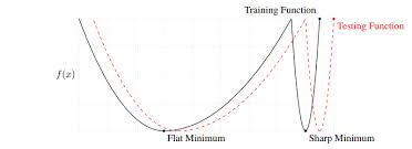
Generally your loss is high dimensional in its parameter space and therefore non-convex. Moreover, the loss itself is usually Lipschitz continuous with a large constant $L$, which leads to the existence of not only local but also sharp minima.

Choosing a learning rate then necessarily depends on both $L$ and the initialization. For a very large $L$, you could still converge with a large learning rate (as opposed to the convex case), as long as the initialization is within a neighbor of a decent flat minima.