Support Vectors of SVM

Question

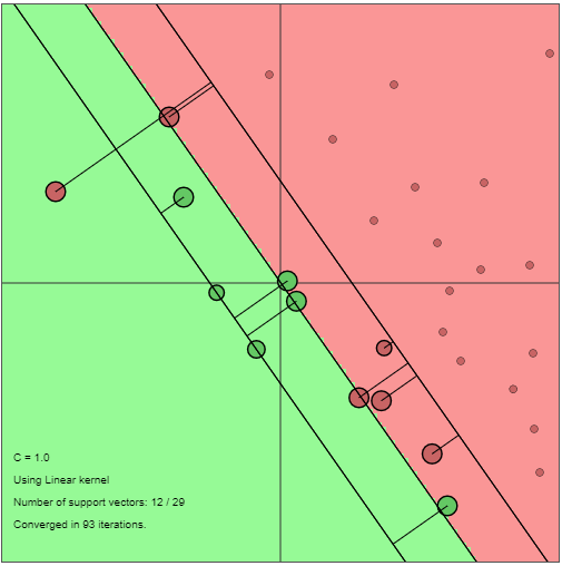
I have read somewhere that the value of slack variables of support vectors is not 0. Does that mean the points lying in the wrong region e.g a positive point lying in the negative region will also be a support vector? I have attached one picture as well which shows that points lying in the wrong region also support vectors. I am looking for an explanation of this phenomenon

Answer 1

Yes, they are support vectors. This is because they contribute (or serve as support) in the computation of the hyperplane that separates the positive and negative regions. This hyperplane is given by:

$$\mathbf{w}^T x + b = 0 $$

Where $x$ is our $\text{n-dimensional}$ input vector that contains the $n$ features of our problem (the input samples during the learning process), and $b$ and $\mathbf{w} = (w_1,w_2,...,w_n)^T$ are the parameters that are optimized. More concretely, $b$ is the intercept of the hyperplane and $(w_1,w_2,...,w_n)^T$ is its normal vector (justification in Mathworld).

But why the misclassified points contribute?

More detailed justifications can be found in the Andrew Ng notes about SVM which I recommend.

To understand why they contribute, we need to have a look at the cost function, $J$, that is used when the data is not linearly separable, like the case of the question (this cost function is also used to prevent the influence of outliers): $$J = \frac{1}{2}\Vert \mathbf{w}\Vert^2 + C \sum_{i=1}^m \xi_i$$ $$\text{subject to}\begin{cases} y^{(i)}(\mathbf{w}^Tx^{(i)}+b)\geq 1-\xi_i, \,\,\,\,\,\,\,\,\,\, i = 1,...,m\\ \xi_i \geq 0 \end{cases}$$ Where $\xi_i$ is the slack of the input sample $x_i$, being $\xi_i = 0$ only when the input sample $x_i$ is correctly classified and presents a functional margin $\geq1$.

In order to solve this in a efficient way, it can be proved that by applying the Lagrange duality to the problem presented before (minimizing $J$ w.r.t. $\mathbf{w}$ and $b$), we end up with a equivalent problem of maximizing the next function w.r.t. $\alpha$: $$ \max_{\alpha}\,\,\,\, \sum_{i=1}^m\alpha_i - \frac{1}{2}\sum_{j=1}^m\sum_{i=1}^my^{(i)}y^{(j)}\alpha_i\alpha_jx_ix_j$$ $$\text{subject to}\begin{cases} 0\leq \alpha_i\leq C, \,\,\,\,\,\,\,\,\,\, i = 1,...,m\\ \sum_{i=1}^m\alpha_iy^{(i)}=0 \end{cases}$$

Where each $\alpha_i$ is the Lagrange multiplier associated with the input sample $x_i$.

Furthermore, it can be proved that, once we have determined the optimal values of the Lagrange multipliers, the normal vector of the hyperplane can be computed by: $$ \mathbf{w}=\sum_i^m \alpha_i y^{(i)}x^{(i)}$$

Now we can see that only the vectors with an associated value of $\alpha_i\neq0$ will contribute to the computation of the hyperplane. This vectors are support vectors.

Now the question is: When $\alpha_i \neq 0$?

As explained in the notes linked above, the values of $\alpha_i \neq 0$ are derived from the KKT conditions which are needed to be satisfied in order to find the values of $\alpha_i$ that minimize our cost function. These are:

1. $\alpha_i = 0 \implies y^{(i)}(\mathbf{w}^Tx^{(i)}+b)\geq 1$
2. $\alpha_i = C \implies y^{(i)}(\mathbf{w}^Tx^{(i)}+b)\leq 1$
3. $0<\alpha_i < C \implies y^{(i)}(\mathbf{w}^Tx^{(i)}+b)= 1$

So, in conclusion the vectors (samples) that lie on the margins (condition number 3 and condition number 2 when $=1$), the vectors that are correctly classified but lie between the margins and the hyperplane (condition number 2 when $<1$) and the vectors that are misclassified (also condition number 2 when $<1$) are the ones with $\alpha_i \neq0$ and therefore contribute to the computation of the hyperplane $\rightarrow$ they are support vectors.