Same SVM configuration, same input data gives different output using Matlab and scikit-learn implementation of SVM, in a classification problem

Question

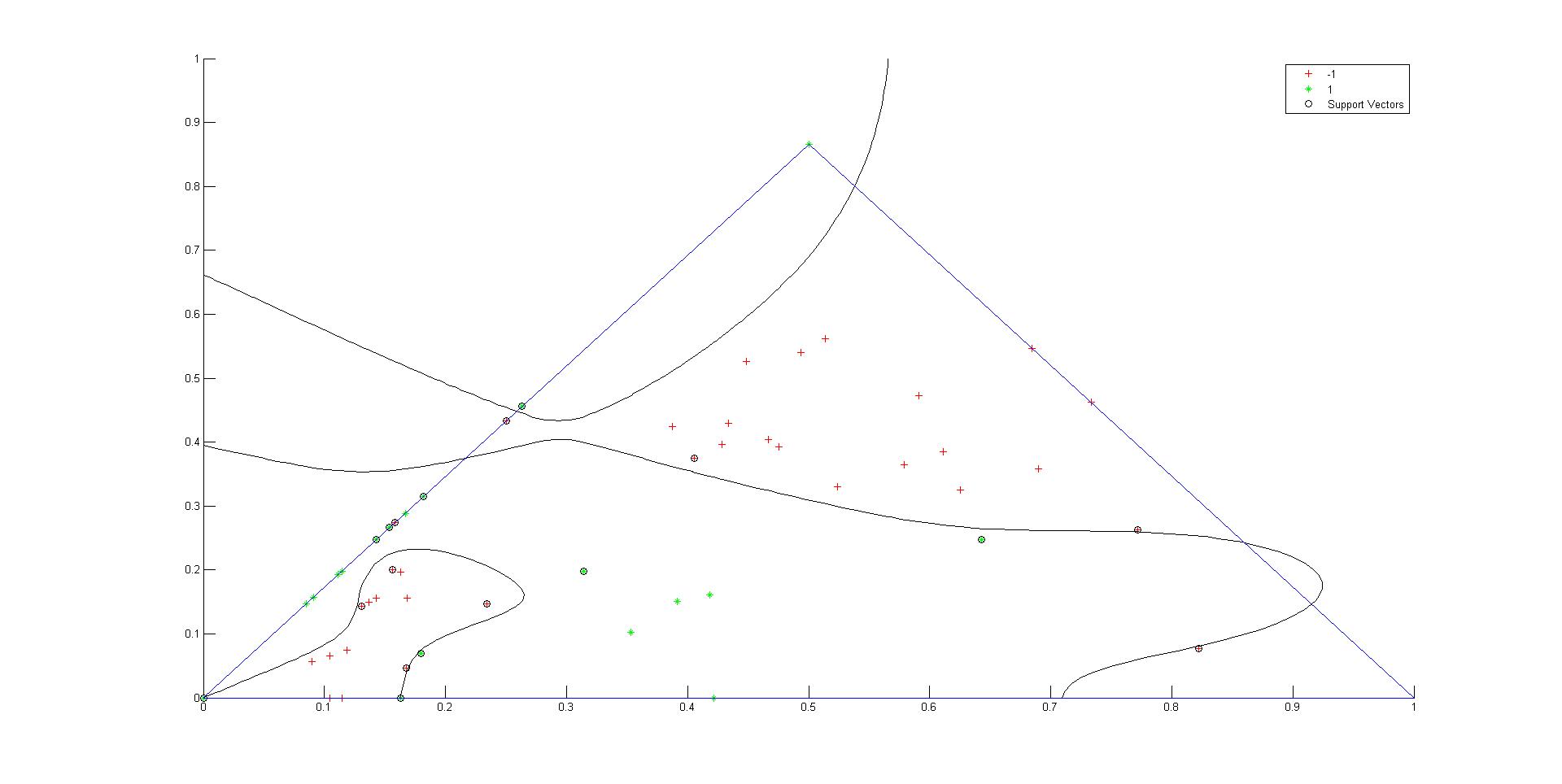
I have a classification problem with 60 data points in a 2-dimensional feature space. The data originally is divided into 2 classes. Earlier I was using Statistics Toolbox of Matlab so it was giving me fairly good results.It was giving 1 false negative and no false positive.

I used the following code:

SVMstruct = svmtrain(point(1:60,:),T(1:60),'Kernel_Function','polynomial','polyorder',11,'Showplot',true);

I am using a polynomial kernel and with polynomial order of 11.

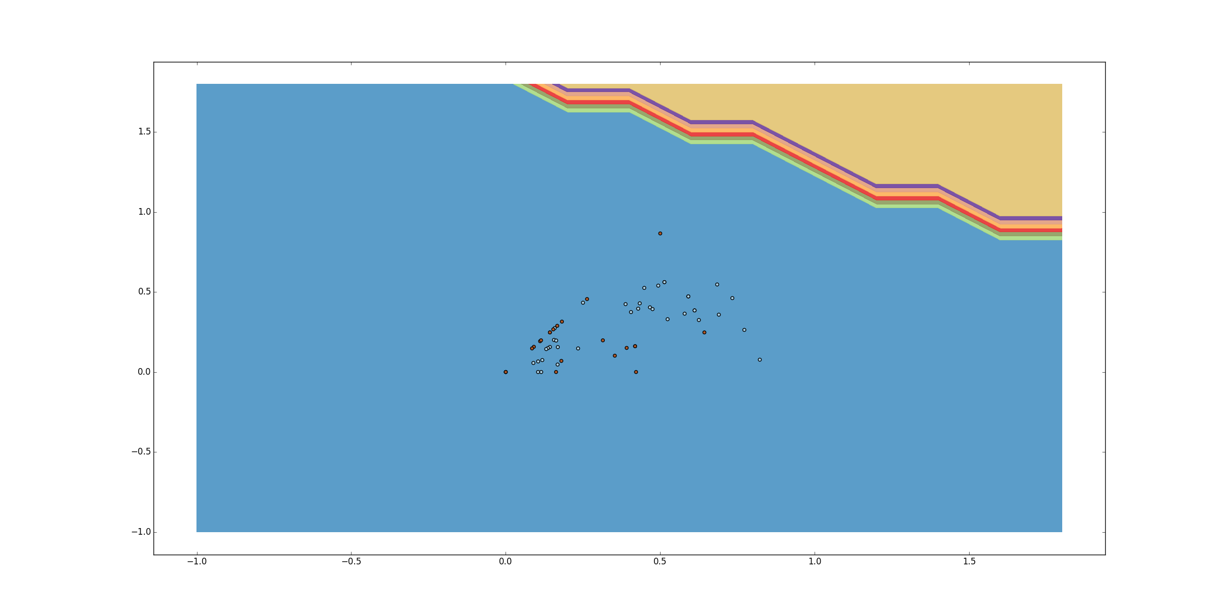
But when I use same kernel configuration in scikit-learn SVC it does not gives the same result rather it gives very undesirable result with classifying all of them to single class.

I am using it as

svc = svm.SVC(kernel='poly', degree=11, C=10)

I have used with many values of C too. No major difference.

Why there is so much difference in results ? How can I get same result as I got using Matlab ? For me it is compulsory to do with python-scikit.

Answer 1

You have to be sure that the algorithm is the same and the kernel functions are really the same. If you look at this python documentation page for kernels in scikit learn you will see there a description of poly kernel.

Notice that you have a gamma and a degree. Gamma is by default 'auto' which is evaluated at 1/n_samples. For the same kernel you have 'coef0' (a great name for a parameter), which is used in poly as the free term. I do not know how matlab put this values as defaults, but the usual formula for poly kernel in literature I found it to be $poly(x_1, x_2) = (<x_1,x_2> + 1)^{d}$. So no gamma and the free term is $1$. I think matlab uses that. (Anyway I found the 'improvements' in scikit learn to have a not so good smell).

Also in this SVC documentation page they state that there is a parameter called shrinking. I really do not know it's effect, but its auto, which means is enabled. Might be an issue.

Later edit:

I found this documentation page for svm in matlab which describes the kernel in the way I stated (no degree, free term with $1$). Also it states that 'SMO' is used by default, make it sure you use 'SMO' in python also.

On the other hand you have to understand that these kind of algorithms are solved by optimization methods which are usually iterative and to save some memory, or cycles their implementations can be different in small details, which will almost produce different results. I agree however that the results should be similar.

Answer 2

SVC Parameters:

What prompted you to use a polynomial kernel? There are cases where this might make sense, but it certainly wouldn't be my first choice. A radial basis function is likely a better fit, which is why it is the default in SKLearn. Step back a minute and take in the big picture perspective. Does your human mind want to create a decision surface using an 11th order polynomial given the points that you showed? It looks like there are a couple islands of white points in your second image that could easily be wrapped with two Gaussian functions aka radial basis functions.

What does the SVC with only default parameters do? I've seen plenty of cases where a regularization parameter as high as 10 or 100 is needed, but you haven't spoken to the cross validation procedure you used to arrive at $C=10$, so I wonder how you got there.

I suggest running SVC with default parameters and seeing what this returns. Then maybe try tuning gamma (this is effectively the buffer zone between the decision surface and points around it) and C (this is the regularization term that controls overfitting aka high variance).

Hope this helps!

Answer 3

I am clueless about the difference coming both the implementation yet, but found how to find a decision boundary for the problem.

At First step I scaled the data to a range [0,100] which earlier was [0,1] for the input. (Still do not know why scaling creates a difference)

And then used a RBF kernal with low gamma and high C value.

svc = svm.SVC(kernel='rbf', gamma=.004, C=1000).

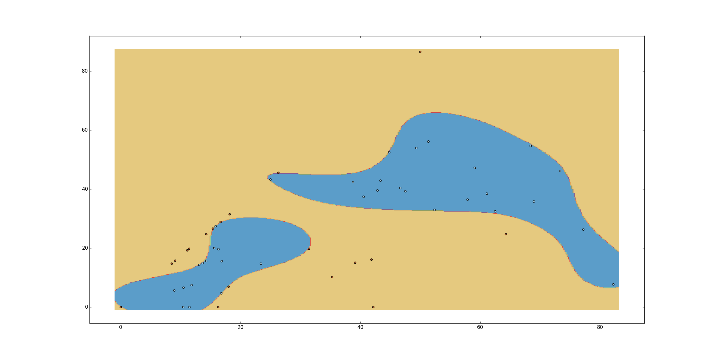
This gives me the following result.