2
$\begingroup$

I'm performing some simulations, and at the end I get a CSV file with three columns. One column holds the values for the x-axis, which was also input to the simulation and theoretical calculations, second one holds theoretically expected values, and the other column holds the values obtained by the simulation. I was planning to plot something like this:

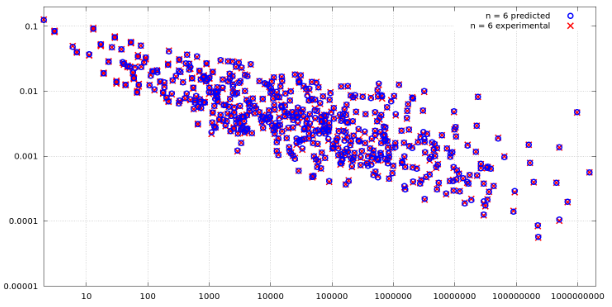
enter image description here

But that does not look good in my case, as the values in y-axis normally keep doubling, and the values for the x-axis exponentially increase, so most of the points end up getting collected at the lower left part, near the intersection of x-axis and y-axis of the plot. Therefore, I need a different way to plot my data, which will be more visually appealing and inform how close the simulation results are to the theoretical expected ones. For example, some of my values can be seen below (and they keep increasing in such a way):

x         = [2, 4, 8, 16, 32, 64] # partially removed for brevity
expected  = [47.9995, 95.9783, 191.9127, 383.9708, 767.8831] # partially removed for brevity 
simulated = [48, 96, 191.8, 383.8, 767.4] # partially removed for brevity

What is a good way to plot such a data that doubles in the y-axis and exponentially increases on the x-axis all the time, and to view how similar the two datasets actually are?

$\endgroup$
7
  • $\begingroup$ Plotting the logarithm of x with the difference between the actual and simulated values will do? $\endgroup$
    – Aditya
    Commented Mar 5, 2018 at 18:12
  • $\begingroup$ @Aditya You mean to take logarithm of every element in x array, and take element-wise difference of elements in expected and simulated arrays? $\endgroup$
    – terett
    Commented Mar 5, 2018 at 18:13
  • $\begingroup$ Exactly but it seems that it will be depending on max(x), Can you add some more of x or tell us the order of x's $\endgroup$
    – Aditya
    Commented Mar 5, 2018 at 18:20
  • $\begingroup$ @Aditya I goes as much as 11-12 digit numbers. $\endgroup$
    – terett
    Commented Mar 5, 2018 at 18:30
  • $\begingroup$ From your plot, it seemed that your model is doing amazing work but it seems that it's highly accurate as it's even mapping some of them lying here and there(seperate from the main cluster) Why it's so? $\endgroup$
    – Aditya
    Commented Mar 9, 2018 at 4:59

2 Answers 2

2
$\begingroup$

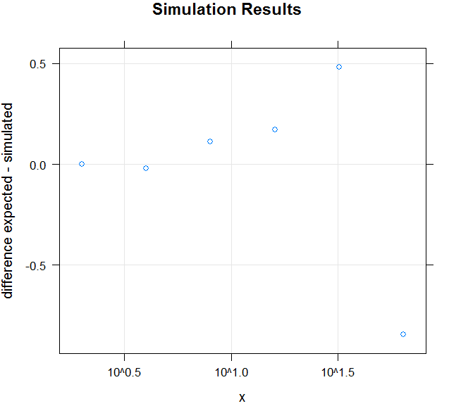
Here is an example of r lattice xyplot using log scale on the x axis and the difference of your two measures I(expected - simulated)

df <- data.frame(
x         = c(2, 4, 8, 16, 32, 64),
expected  = c(47.9995, 95.9783, 
191.9127, 383.9708, 767.8831, 
1457.2771),
simulated = c(48, 96, 191.8, 383.8, 
767.4, 1458.1228))
xy <- xyplot(I(expected - simulated) ~ x ,   
auto.key=TRUE,
data =  df ,    type=c("p","g"),
scales=list(x=list(log = 10) ),   
ylab="difference expected - simulated", xlab="x", main="Simulation Results" )
print (xy)

Note, that I added a 6th result to your sample data,that was missing.

enter image description here

$\endgroup$
0
2
$\begingroup$

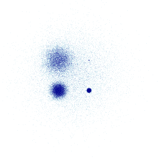
Here we have 50000 points, 10000 in each of five categories with associated numerical values.

Instead of using Logarithms, you can also use O( log* N ) is "iterated logarithm":

In computer science, the iterated logarithm of n, written log* n (usually read "log star"), is the number of times the logarithm function must be iteratively applied before the result is less than or equal to 1.

Checkout Datashader (This is what you Need)

Reference Notebook

Generating Something Random(you will get the idea)

import pandas as pd
import numpy as np

np.random.seed(1)
num=10000

dists = {cat: pd.DataFrame(dict(x=np.random.normal(x,s,num),
                                y=np.random.normal(y,s,num),
                                val=val,cat=cat))
         for x,y,s,val,cat in 
         [(2,2,0.01,10,"d1"), (2,-2,0.1,20,"d2"), (-2,-2,0.5,30,"d3"), (-2,2,1.0,40,"d4"), (0,0,3,50,"d5")]}

df = pd.concat(dists,ignore_index=True)
df["cat"]=df["cat"].astype("category")
df.tail()

cat val x y 49995 d5 50 -1.397579 0.610189 49996 d5 50 -2.649610 3.080821 49997 d5 50 1.933360 0.243676 49998 d5 50 4.306374 1.032139 49999 d5 50 -0.493567 -2.242669

%time tf.shade(ds.Canvas().points(df,'x','y'))

Output Image

The Picture Clearly Shows 5 Normal Distributions

$\endgroup$

Your Answer

By clicking “Post Your Answer”, you agree to our terms of service and acknowledge you have read our privacy policy.

Not the answer you're looking for? Browse other questions tagged or ask your own question.