Why could my SVR prediction be offset, but still follow the actual pattern?

Question

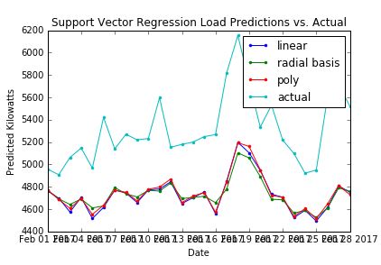
I am running an SVR prediction on some time series data, and I am receiving this weird offset between my actual and predicted values.

I found this SVM Regression lag post, that mentions adding a lag of 2 data points behind, instead of one. However, I am not sure how to incorporate that into my code (which I've included below).

Does anyone have any ideas on why my predicted vs. actual is offset in this manner?

My code is as follows:

#! /usr/bin/python

import math
import statistics
import visualizer
import numpy as np
from datagen import constructData
from sklearn import svm

# Applies Support Vector Regression to the electricity dataset,
# prints out the accuracy rate to the terminal and plots
# predictions against actual values
def suppVectorRegress():

    kernelList = ["linear","rbf",polyKernel]
    names = ["linear","radial basis","poly"]
    preds = []

    # Retrieve time series data & apply preprocessing
    data = constructData()

    cutoff = len(data)-30
    xTrain = data[0][0:cutoff]
    yTrain = data[1][0:cutoff]
    xTest = data[0][cutoff:]
    yTest = data[1][cutoff:]

    # Fill in missing values denoted by zeroes as an average of
    # both neighbors
    statistics.estimateMissing(xTrain,0.0)
    statistics.estimateMissing(xTest,0.0)

    # Logarithmically scale the data
    xTrain = [[math.log(y) for y in x] for x in xTrain]
    xTest = [[math.log(y) for y in x] for x in xTest]
    yTrain = [math.log(x) for x in yTrain]

    # Detrend the time series
    indices = np.arange(len(data[1]))
    trainIndices = indices[0:cutoff]
    testIndices = indices[cutoff:]
    detrended,slope,intercept = statistics.detrend(trainIndices,yTrain)
    yTrain = detrended

    for gen in range(len(kernelList)):

        # Use SVR to predict test observations based upon training observations
        pred = svrPredictions(xTrain,yTrain,xTest,kernelList[gen])
        # Add the trend back into the predictions
        trendedPred = statistics.reapplyTrend(testIndices,pred,slope,intercept)
        # Reverse the normalization
        trendedPred = [np.exp(x) for x in trendedPred]
        # Compute the NRMSE
        err = statistics.normRmse(yTest,trendedPred)

        print ("The Normalized Root-Mean Square Error is " + str(err) + " using kernel " + names[gen] + "...")

        preds.append(trendedPred)

    names.append("actual")
    preds.append(yTest)

    # Change the parameters 2017,2,1 based on the month you want to predict.
    visualizer.comparisonPlot(2017,2,1,preds,names,plotName="Support Vector Regression Load Predictions vs. Actual", 
        yAxisName="Predicted Kilowatts")

# Construct a support vector machine and get predictions
# for the test set
# Returns a 1-d vector of predictions
def svrPredictions(xTrain,yTrain,xTest,k):
    clf = svm.SVR(C=2.0,kernel=k)
    clf.fit(xTrain,yTrain)
    return clf.predict(xTest)

# A scale invariant kernel (note only conditionally semi-definite)
def polyKernel(x,y):
    return (np.dot(x,y.T)+1.0)**0.95

if __name__=="__main__":
    suppVectorRegress()

Answer 1

Two things that come to my mind:

A) - have you compared the distributions with a Kolgomorov Smirnov Test or similar - (aka: are they really the same. Sure there is the big spike but besides its not that similar (by eye))

B) - Are training and test in the same magnitudes for the input data? If they are not this might confuse your SVR.