Uncertainty about shape of ROC curve

Question

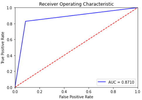
I am working on a binary classification and the plotted ROC curves that I am using for evaluation together with AUC, have seemed strange to me. Here is an example.

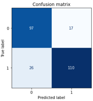
I understand that ROC is a visual representation of the true positive rate versus the false positive rate. When plotting the confusion matrix I can see there are significant number of false negatives and false positives alike:

I fail to understand how it is possible that the ROC curve only has a single break point. My question therefore is: What is the reason for ROC having such a shape instead of the typical smooth(er) monotonically increasing shape?

I tried playing around with the n_iter argument of RandomizedSearchCV, with the n_splits of StratifiedKFold and with the classifier estimator used (LogisticRegression(), RandomForestClassifier()).

Full reproducible code:

from sklearn.datasets import make_classification
from sklearn.linear_model import LogisticRegression
from sklearn.ensemble import RandomForestClassifier 
from sklearn.model_selection import train_test_split, StratifiedKFold, RandomizedSearchCV
from sklearn.metrics import ConfusionMatrixDisplay, confusion_matrix, roc_curve

random_seed = 12345
X, y = make_classification(n_samples=1000, n_features=5, n_classes=2)
X_train, X_test, y_train, y_test = train_test_split(X, y, random_state=random_seed)
cv = StratifiedKFold(n_splits=10, shuffle=True, random_state=random_seed)

search_output = RandomizedSearchCV(
    estimator = RandomForestClassifier(max_depth=10), 
    param_distributions = {'n_estimators': np.arange(100, 501, 50)},
    n_iter = 3, 
    scoring = 'roc_auc', 
    n_jobs = -1,
    cv = cv, 
    refit = True, 
    verbose = 1, 
    return_train_score = True, 
    random_state = random_seed  
).fit(X_train, y_train)

best_model = search_output.best_estimator_

y_preds = best_model.predict(X_test)

fpr, tpr, threshold = metrics.roc_curve(y_test, y_preds)
roc_auc = metrics.auc(fpr, tpr)
print(f"ROC-AUC: {roc_auc}.")
plt.title('Receiver Operating Characteristic')
plt.plot(fpr, tpr, 'b', label = f'AUC = {roc_auc:.4f}')
plt.legend(loc = 'lower right')
plt.plot([0, 1], [0, 1],'r--')
plt.xlim([0, 1])
plt.ylim([0, 1])
plt.ylabel('True Positive Rate')
plt.xlabel('False Positive Rate')
plt.show()

cm = confusion_matrix(y_test, y_preds, normalize=None)
fig, ax = plt.subplots(figsize=(4, 4))

disp = ConfusionMatrixDisplay(confusion_matrix=cm)
disp.plot(cmap="Blues", values_format=".0f", ax=ax, colorbar=False)

plt.title("Confusion matrix")
plt.show()

Answer 1

Oops. I found the reason!

The shape of ROC returned by the roc_curve depends on the number of unique values that are input to roc_curve. In my case I was getting only 3 points on the ROC curve. The mistake I made was that roc_curve needs an y_score argument, not an y_pred argument: this is the probability score of each predictions. As such instead of:

y_preds = best_model.predict(X_test)

fpr, tpr, threshold = metrics.roc_curve(y_test, y_preds)
roc_auc = metrics.auc(fpr, tpr)

I should have written:

y_preds = best_model.predict(X_test)
y_pred_probas = best_model.predict_proba(X_test)[:,1]

fpr, tpr, threshold = metrics.roc_curve(y_test, y_pred_probas)
roc_auc = metrics.auc(fpr, tpr)

(Note that predict_proba() returns a 2d numpy array with probability values corresponding to each observation where first column shows the probabilities of the given observation being in class "0" while second column shows the probabilities that a given observation is in class "1". Since for binary classification the two columns are redundant, we only need the column corresponding for class "1" to plot the ROC.)

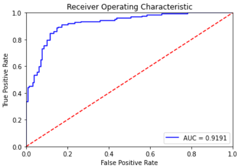
And this will now yield a nice ROC curve as expected:

Answer 2

Your confusion matrix and ROC curve come from distinct notions. The confusion matrix is calculated for a single threshold. Your model returns numbers (looks like probability values), and the threshold determines the categories to which the numbers correspond. A common choice is to use $0.5$ for a model that outputs probability values. In all likelihood, this is the threshold being used in your software. Depending on the particulars of your problem, a different threshold might be much more appropriate, or the most appropriate threshold might be not to use any threshold at all and directly evaluate the probability outputs. I will include two links to further reading on doing away with thresholds.

https://www.fharrell.com/post/class-damage/ https://www.fharrell.com/post/classification/

In a ROC curve, you calculate what’s going on at all possible thresholds and plot the resulting sensitivity and specificity values. Set the threshold at $0.01$; calculate sensitivity and specificity; plot that point. Set the threshold at $0.02$, calculate the sensitivity and specificity; plot that point.